Towards a Theory of Generalization in Reinforcement Learning: guest lecture by Sham Kakade

Windows On Theory 2021-04-24

Scribe notes by Hamza Chaudhry and Zhaolin Ren

Previous post: Natural Language Processing – guest lecture by Sasha Rush Next post: TBD. See also all seminar posts and course webpage.

See also video of lecture. Lecture slides: Original form: main / bandit analysis. Annotated: main / bandit analysis.

Sham Kakade is a professor in the Department of Computer Science and the Department of Statistics at the University of Washington, as well as a senior principal researcher at Microsoft Research New York City. He works on the mathematical foundations of machine learning and AI. He is the recipient of the several awards, including the ICML Test of Time Award (2020), the IBM Pat Goldberg best paper award (in 2007), and the INFORMS Revenue Management and Pricing Prize (2014).

Sham is writing a book on the theory of reinforcement learning with Agarwal, Jiang and Sun.

Introduction:

Reinforcement learning has found success in a great number of fields because it is a very “natural framework” for interactive learning. It is based around the notion of experimenting with different behaviors in one’s environment and learning from mistakes to identify the optimal strategy. However, there is a lack of understanding regarding how to best optimize reinforcement learning algorithms when there is uncertainty about the agent’s environment and potential rewards. Therefore, it is important to develop a theoretical foundation about this to study generalization in reinforcement learning. The primary question these notes will address is as follows:

What are necessary representational and distributional conditions that enable provably sample-efficient reinforcement learning?

We will answer this question in the following parts.

Part I: Bandits & Linear Bandits “Bandit problems” correspond to RL where the environment is reset in each step (horizon H=1). This captures the aspect of having an unknown reward function of RL, but does not capture the aspect of a changing environment based on agent’s actions. This part will be based on the papers Dani-Hayes-Kakade 08 and Srinivas-Kakade-Krause-Seeger 10
Part II: Lower Bounds RL is very much not a solved problem in neither theory nor practice. Even the RL analog of linear regression, when the expected reward is a linear function of the actions, is not solved. We will see that this is for a good reason: there is an exponential lower bound on the number of steps it takes to find a nearly-optimal policy in this case. This part is based on the recent paper Weisz-Amortila-Szepesvári 20 and the follow-up Wang-Wang-Kakade 21
Interlude: Do these lower bounds matter in practice?
Part III: Upper Bounds Given the lower bound, we see that to get positive results (aka upper bounds on the number of steps) we need to make strong assumptions on the structure of reqards. There have been a number of incomparable such assumptions used, and we will see that there is a way to unify them. This part is based on the recent paper Du-Kakade-Lee-Lovett-Mahajan-Sun-Wang 21

Before all of these parts, we will start by introducing the general framework of Markov Decision Processes (MDPs) and do a quick tour of generalization for static learning and RL.

Markov Decision Processes: A Framework for Reinforcement Learning

We have an agent in an environment at state $s_t$ that takes some action $a_t$ which will observe some reward $r_{t}$ and update the environment to state $s_{t+1}$ .

The following are some key terms that we will need throughout the rest of the notes:

State Space, Action Space, Policy: We denote the state space as $\mathcal{S}$ , and the action space as $\mathcal{A}$ . A policy $\pi$ is a mapping from states to actions: $\pi: \mathcal{S} \to \mathcal{A}$
Trajectory: The sequence of states, actions, rewards an agent sees for a horizon of $H$ timesteps. $(s_1, a_1, r_1, s_2, a_2, r_2, \dots, s_{H}, a_{H}, r_{H})$
State Value at time $h$ : The expected cumulative reward starting from state $s$ and using policy $\pi$ afterwards.
$V_h^\pi(s) = \mathbb{E} \left[ \sum_{t=h}^{H} r_t \vert s_h = s \right]$
State Action Value at time $h$ : The expected cumulative reward given a state-action tuple $(s,a)$ starting from time $h$ and using policy $\pi$ afterwards. $Q_h^\pi(s,a) = \mathbb{E} \left[ \sum_{t=h}^{H} r_t \vert s_h = s, a_h = a \right]$
Optimal value and state-value function: we define an optimal policy by $\pi^\star$ , and the associated optimal $Q$ -function and value function by $Q^\star$ and $V^\star$ respectively (or equivalently, $Q^{\pi^\star}$ , $V^{\pi^\star}$ ). Note that $Q^\star$ and $V^\star$ can be defined via the Bellman optimality equation as follows:

$V_h^\star(s) = \max_{a \in \mathcal{A}} Q_h^\star(s,a)$

$Q_h^\star(s,a) = \mathbb{E}\left[R_h(s,a) + V_{h+1}^\star(s_{h+1}) \mid s_h = s, a_h = a \right]$

where we additionally define $V_{H+1}(s) = 0$ for all $s \in \mathcal{S}$ .

Goal: To find a policy $\pi$ that maximizes the cumulative H-step reward $V_1^\pi(s)$ starting from an initial state $s$ with a horizon $H$ . In the episodic setting, one starts at state $s_1$ , acts for $H$ steps, and then repeats.

Challenges in Reinforcement Learning

There are three main challenges that we face in reinforcement learning

Exploration: The total size and states of the environment may be unknown.
Credit Assignment: We need to assign rewards to actions even if the rewards are delayed.
Large State/Action Spaces: We face the curse of dimensionality.
- OpenAI 2019 Dexterous Robotic Hand Manipulation

We will deal with these problems by framing them in terms of generalization.

Part 0: A Whirlwind Tour of Generalization

Provable Generalization in Supervised Learning

As we have seen in the first lecture of this course, generalization is possible in the supervised learning setting, when the data follows an i.i.d distribution. Specifically we have the following bound

Occam’s Razor Bound (Finite Hypothesis Class): To learn a policy that is $\epsilon-$ close to the best policy in a hypothesis class $\mathcal{F}$ , we need a number of samples that is $\mathcal{O} (\log(|\mathcal{F}|) / \epsilon^2)$ .

This means we can try lots of things on our data to see which hypotheses are $\epsilon$ -best. To handle infinite hypothesis classes, we can replace $\log |\mathcal{F}|$ with various other “complexity measures” to obtain generalization bounds such as:

VC Dimension: $\mathcal{O} (\text{VC}(\mathcal{F}) / \epsilon^2)$
Classification (Margin Bounds): $\mathcal{O} (\text{margin} / \epsilon^2)$
Linear Regression: $\mathcal{O}(\text{dimension}/\epsilon^2)$
Deep Learning: Algorithm also determines the complexity control

Another way to say this is that in all of these cases, we can bound the generalization gap $\epsilon$ by a quantity of the form $O(\sqrt{d/n})$ where $d$ is some “complexity measure” of the class $\mathcal{F}$ and $n$ is the number of samples.

One reference for these generalization results in the supervised learning setting is the following book by Sanjeev Arora and collaborators.

The key enabler of generalization in supervised learning is data reuse. For a given training set, we can in principle simultaneously evaluate the loss of all hypotheses in our class. For example, given the fixed ImageNet dataset, we can evaluate performance on any classifier. As we will see, this is not a property that will always hold in RL (when it does hold, sample-efficient generalization is likely to follow).

Sample Efficient RL in the Tabular Case with few states and actions (No Generalization involved):

Consider a tabular MDP setting where $S$ , $A$ and $H$ denote the number of states, number of actions and length of the horizon respectively. Suppose we are operating in a setup where $S$ and $A$ are both small. Suppose also that the MDP is unknown.

Our goal in such a setting is to find a $\epsilon$ -optimal policy $\pi$ such that $V_{1}^{\pi}(s_1) \geq V_1^{\pi^\star}(s_1) - \epsilon$ , where $s_1$ is the initial state (for concreteness let’s assume it is deterministic), and $\pi^\star$ is truly an optimal policy for this MDP. Since we assume the number of states and actions to be small, it is possible to explore the entire world, and finding such an $\epsilon$ -optimal policy is in principle possible. We thus do not have to consider any hypothesis class here (so no generalization involved), and can instead seek to be optimal under all possible mappings from states to actions.

Think for example of the following maze MDP, where the state of the world is the cell the agent is in and the action it can take at each state is a move to each of say 4 neighboring cells. Then, if we are able to get to every state and try every action there, we would have learned the world.

In this particular scenario, randomly exploring the world will allow us to learn the world. However, if we consider a modified random exploration strategy, where the probability of going left is significantly larger (say 5 times larger) than the probability of going right, then it will take exponential time to hit the goal state. In general, even for MDPs with small state and action spaces, a purely random exploration approach may be insufficient, as we may not be exploring the world enough. What alternative approach might we then adopt in order to achieve a sample-efficient learning algorithm?

Theorem: (Kearns & Singh ’98). In the episodic setting, $poly(S,A,H,1/\epsilon)$ samples suffice to find an $\epsilon-$ opt policy, where $S$ is the number of states, $A$ is the number of actions, and $H$ is the length of the horizon.

The above breakthrough result was the first to demonstrate that learning an $\epsilon$ -opt policy is possible using just polynomially many samples. The key idea behind this is optimism and dynamic programming. In proving the result, the authors designed an algorithm called the E $^3$ algorithm (Explicit Explore or Exploit). The E $^3$ algorithm adopts a model-based approach, and relies on a “plan-to-explore” mechanism. As we act randomly, we will learn some part of the state space, and having learned this region well, we can thus accurately plan to escape it. This is where optimism comes in, since we give ourselves a bonus for escaping a region we know well.

Based on the Kearns and Singh result, there has been a number of followup works on the tabular MDP setting. One line of work seeks to improve on the precise factors in the sample complexity.

Improvements on the sample complexity:

A General Polynomial Time Algorithm for Near-Optimal Reinforcement Learning / Brafman-Tennenholtz 2002
On the Sample Complexity of Reinforcement Learning – Kakade 2003 (PhD Thesis).
Near-Optimal Regret Bounds for Reinforcement Learning – Jaksch, Ortner, Auer 2010
Posterior sampling for reinforcement learning: worst-case regret bounds – Agrawal Jia 2017

Another line of work seeks to show that Q-learning, a model-free approach, can also achieve similar polynomial complexity, if an appropriate optimism bonus is incorporated.

Provable Q-Learning (+Bonus)

PAC Model-Free Reinforcement Learning – Strehl-Li-Wiewiora-Langford-Littman 2006
Algorithms for Reinforcement Learning – lecture by Szepesv´ari 2009
Is Q-learning Provably Efficient? – Jin Allen-ZhuBubeck Jordan 2018

As the range and technical depth of the above results demonstrate, even in the relatively simple tabular case, the problem is already challenging, and a precise sharp characterization of sample complexity is even more difficult. The chief source of difficulty is the unknown nature of the world (if the world was known, then we can just run dynamic programming).

Provable Generalization in RL:

Ultimately, we want to move beyond small tabular MDPs, where a polynomial dependence in the sample complexity on $S$ is acceptable, and achieve sample-efficient learning in big problems where the space space could be massive. Think for instance of the game of Go.

In such a setting, requiring polynomially (in $S$ ) many samples is clearly unacceptable. This gives rise to the following question.

Question 1: Can we find an $\epsilon-$ opt policy with no $S$ dependence?

In order to do so, it is necessary to reutilize data in some way since we will not be able to see all the possible states in the world. How then might we reuse data to estimate the value of all policies in a policy class $\mathcal{F}$ ? A naive approach is the following:

Idea: Trajectory tree algorithm
Dataset Collection: Choose actions uniformly at random for all H steps in an episode.
Estimation: Uses importance sampling to evaluate every $f \in \mathcal{F}$ .

Theorem: (Kearns, Mansour, & Ng ’00) To find an $\epsilon-$ best in class policy, the trajectory tree algorithm uses $O(A^H\log(|\mathcal{F}|)/\epsilon^2)$ samples.

Observe that when $H = 1$ (i.e. a contextual bandit) this is exactly the kind of generalization bound we saw in the Occam Razor’s bound for supervised learning. Since there may be stochasticity in the MDP, such that $S$ could be infinite or even uncountable, this dependence on $A^H$ is a genuine improvement on the results for the tabular MDP setting which depended polynomially on $S$ . In this sense, this really is a generalization result, since we are learning an $\epsilon$ -best in class policy without having seen the entire world (i.e. all the states in the world). We note that the result only has $\log(\mathcal{F}|)$ dependence on hypothesis class size and similar to the supervised learning setting, there are VC analogues as well. However, we can not avoid the $A^H$ dependence to find an $\epsilon-$ best-in-class policy agnostically (without assumptions on the MDP). To see why, consider a binary tree with $2^H$ -policies and a sparse reward at a leaf node.

This $A^H$ dependence, while unavoidable without further assumptions, is clearly undesirable. This brings us to the following question.

Question 2: Can we find an $\epsilon-$ opt policy with no $S,A$ dependence and $poly(H,1/ \epsilon, \text{"complexity measure"})$ samples?

As we just saw, agnostically we cannot learn an $\epsilon$ -best-in-class policy without an $A^H$ dependence. However, as we will see it is possible when appropriate assumptions are made. But what is the nature of the assumptions under which this kind of sample-efficient RL generalization is possible (when there is no (or mild) dependence on $S$ and $A$ )? What assumptions are necessary? What assumptions are sufficient? We will seek to address these questions.

To do so, we start simple, and first look at the bandits and linear bandits problem, where the horizon $H$ is just 1. Note that this is still an interactive learning problem, just that we reset the episode after one time-step, and that it is an example of a problem with a potentially large action space.

Part 1: Bandits and Linear Bandits

Multi-Armed Bandits:

The multi-armed bandits algorithm is intimately interwoven with the theory of reinforcement learning. It is based around the question of how to allocate T tokens to A “arms” to maximize one’s return:

Some Aspects of the Sequential Design of Experiments – Robbins 1952
Bandit Processes and Dynamic Allocations Indices – Gittins 1979
Asymptotically Efficient Adaptive Allocation Rules – Lai and Robbins 1985

It is a very successful algorithm when $A$ is small. What can we do when $A$ is large?

Large-Action Case:

The bandits have to make a decision regarding which arm to pull. There is a widely used linear formulation of this problem that will assist us in understanding generalization. The linear bandit model is successful in many applications (scheduling, ads, etc.)

Linear (RKHS) Bandits:

Decision: $x_t$ ; Reward: $r_t$ ; Reward model: $r_t = f(x_t) + \text{noise}; f(x) = w^\star \cdot \phi(x)$
The hypothesis class $\mathcal{F}$ is a set of linear/RKHS functions (an overview of RKHS, which stands for Reproducing Kernel Hilbert Space, can be found here).

Linear/Gaussian Process Upper Confidence Bounds (UCB):

The principle underlying the Linear Bandits algorithm is optimism in the face of uncertainty: Pick an input that maximizes the upper confidence bound:

$x_t = \text{arg}\max_{x \in D} \mu_{t-1}(x) + \beta_t \sigma_{t-1}(x).$

Note that $\mu_{t-1}$ is the best estimate of the ground-truth and $\sigma_{t-1}$ is a standard deviation that we have to estimate. In choosing the term $\beta_t$ , we have to navigate a trade-off between exploration and exploitation. As we can see, this algorithm will only pick plausible maximizers.

Regret of Linear-UCB / Gaussian Process-UCB (Generalization in Action Space)

Theorem: (Dani, Hayes, & K. ’08), (Srinivas, Krause, K., & Seeger ’10). Assuming $\mathcal{F}$ is an RKHS (with bounded norm), if we choose $\beta_t$ “correctly”, then the regret satisfies $\frac{1}{T} \sum_{t=1}^T[f(x^\star) - f(x_t)] = \tilde{\mathcal{O}} \left( \sqrt{\frac{\gamma_T}{T}} \right),$ where $\tilde{\mathcal{O}}$ hides logarithmic terms, and

The key complexity concept here is “Maximum Information Gain”: $\gamma_T$ , which one can think of as the “effective dimension,” determines the regret because $\gamma_T \approx d \log T$ for $\phi$ in $\mathbb{R}^d$ . Here are some relevant papers for further understanding regret, which is the difference between the reward of a possible action and the reward of an action that has been taken.

Finite-time Analysis of the Multiarmed Bandit Problem – Auer Cesa-Bianchi Fischer 2002
Improved Algorithms for Linear Stochastic Bandits – Abbasi-yadkori, Pál, Szepesvári 2011

Linear Upper Confidence Bound Analysis

Handling Large Action Spaces

On each round, we must choose a decision $x_t \in D \subset R^d$ . This yields a reward $r_t \in [-1,1]$ , where

$\mathbb{E}[r_t | x_t = x] = \mu^\star \cdot x \in [-1,1].$

Above, $\mu^\star$ is an unknown weight vector and $x$ may be replaced by $\phi(x)$ if we have access to such a representation. Note that this tells us that the conditional expectation of $r_t$ upon $x_t$ is linear. We have the a corresponding i.i.d. noise sequence $\eta_t = r_t - \mu^\star \cdot x_t$ . If $(x_0, \dots, x_{T-1})$ are our decisions, then our cumulative regret in expectation is

$R_T = T(\mu^\star \cdot x^\star) - \sum_{t=0}^{T - 1} \mu^\star \cdot x_t$

where $x^\star\in D$ is an optimal decision for $\mu^\star$ , i.e.

$x^\star \in \text{arg}\max_{x \in D} \mu^\star \cdot x$

LinUCB and the Confidence Ball

After t rounds, we can define our uncertainty region $\text{BALL}_t$ with center $\hat{\mu_t}$ and shape $\Sigma_t$ using the $\lambda-$ regularized least squares solution:

$\hat{\mu_t} = \text{arg}\min_\mu \sum_{\tau = 0}^{t-1} \left\| \mu \cdot x_\tau - r_\tau \right\|_2^2 + \lambda \left \| \mu \right\|_2^2,$
$\Sigma_t = \lambda I + \sum_{\tau = 0}^{t-1} x_\tau x_\tau^\top \text{, with } \Sigma_0 = \lambda I,$
$\text{BALL}_t = \left\{ \mu: (\hat{\mu_t} - \mu)^\top \Sigma_t (\hat{\mu_t} - \mu) \leq \beta_t \right\},$
$\beta_t$ is a parameter of the algorithm and $\Sigma_t$ determines how accurately we know $\hat{\mu_t}$

The LinUCB Algorithm can be understood as follows: For $t = 0,1,\dots$

Execute $x_t = \text{arg}\max_{x \in D} \max_{\mu \in \text{BALL}_t} \mu \cdot x$
Observe the reward $r_t$ and update $\text{BALL}_{t+1}$

LinUCB Regret Bound

As the following theorem shows, the regret $R_T \leq \tilde{\mathcal{O} }(d\sqrt T)$ is sublinear with polynomial dependence on $d$ and no dependence on the cardinality $|D|$ of the decision space $D$ .

Theorem (regret): (Dani, Hayes, Kakade 2009). Suppose we have bounded noise $|\eta_t|$ ; $|| \mu^\star || \leq W$ ; $||x|| \leq B$ , for $x\ \in D$ . Set $\lambda = \sigma^2/W^2, \quad \beta_t := c_1 \sigma^2\left(d \log\left(1 + \frac{TB^2}{d}\right) + \log(1 /\delta)\right).$ Then, with probability greater than $1 - \delta$ , for all $t \geq 0$ , $R_T \leq c_2 \sigma \sqrt{T} \left ( d \log\left(1 + \frac{TB^2}{d \sigma^2}\right) + \sqrt{\log(1 /\delta)}\sqrt{d \log\left(1 + \frac{TB^2}{d}\right)} \right),$ where $c_1,c_2$ are absolute constants.

To prove the regret theorem above, we will require the following two lemmas.

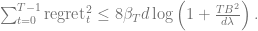
Lemma 1 (Confidence): Let $\delta > 0$ . We have that $Pr(\forall t, \mu^\star \in \text{BALL}_t) \geq 1 - \delta.$

Lemma 2 (Sum of Squares Regret Bound): Define $\text{regret}_t = \mu^\star \cdot x^\star - \mu^\star \cdot x_t$ . Suppose $\beta_t \geq 1$ is increasing and that for all $t$ , we have $\mu^\star \in \text{BALL}_t$ . Then, $\sum_{t=0}^{T-1} \text{regret}_t^2 \leq 8 \beta_T d \log \left ( 1 + \frac{TB^2}{d\lambda} \right ).$

We note that Lemma 2 actually depends on Lemma 1, since it assumes that $\mu^\star \in \text{BALL}_t$ for each $t$ , a property that Lemma 1 tells us happens with probability at least $1-\delta$ . We defer the proofs of the two lemmas to later, and first show why they can be used to prove the regret theorem.

Proof of regret theorem: Using the two lemmas above along with the Cauchy-Schwarz inequality, we have with probability at least $1 - \delta$ that

$R_T = \sum_{t=0}^{T-1} \text{regret}_t \leq \sqrt{T \sum{t=0}^{T-1} \text{regret}_t^2} \leq \sqrt{8 T \beta_T d \log \left( 1 + \frac{TB^2}{d\lambda} \right)}.$

The rest of the proof follows from our chosen value of $\beta_T$ . $\square$

We now proceed to sketch out the proofs of Lemma 1 (confidence bound) and Lemma 2 (sum of squares regret bound). We begin with showing why Lemma 2 holds.

Analysis and proof of Lemma 2 (sum of squares regret bound)

Our first auxilliary result bounds the pointwise width of the confidence ball.

Lemma (pointwise width of confidence ball). Let $x \in D$ . Consider any $\mu \in \text{BALL}_t$ . Then, $| (\mu - \hat{\mu}_t)^\top x| \leq \sqrt{\beta_t x^\top \Sigma_t^{-1}x}.$

Proof. We have

where the first inequality follows from Cauchy-Schwarx and the second (i.e last) inequality holds by the definition of $\text{BALL}_t$ and our assumption that $\mu \in \text{BALL}_t.$ $\square$

Let us now define

$w_t := \sqrt{x_t^\top \Sigma_t^{-1}x_t},$

which we can think of as the “normalized width” at time $t$ in the direction of our decision. We have the following bound on the instantaneous regret $\text{regret}_t$ .

Lemma (instantaneous regret lemma). Fix $t \leq T$ . If $\mu^\star \in \text{BALL}_t$ , then $\text{regret}_t \leq 2 \min (\sqrt{\beta_t}w_t, 1) \leq 2 \sqrt{\beta_t} \min(w_t,1).$

Proof. The basic idea is to use “optimism”. Let $latex \tilde{\mu} \in \text{BALL}t&bg=ffffff$ denote the vector maximizing the dot product $\hat{\mu}^\top x_t$ . By choice of $x_t$ , $latex \tilde{\mu}^\top x_t = \max{\mu \in \text{BALL}_t} \max{x \in D}\mu^\top x \geq (\mu^\star)^\top x^\star&bg=ffffff$, where the inequality used the hypothesis that $\mu^\star \in \text{BALL}_t$ . This manifestation of “optimism” is crucial, since it tells us that the “ideal” reward we think we can get at time $t$ exceeds the optimal expected reward $(\mu^\star)^\top x^\star$ . Hence,

where the last step follows from the pointwise width lemma (note $\tilde{\mu}$ is in $\text{BALL}_t$ and $\mu^\star$ is assumed to be $\text{BALL}_t$ by the hypothesis in Lemma 2). Since in the linear bandits setup we assumed that $\mu^\star \cdot x \in [-1,1]$ for all $x \in D$ , the simple bound $\text{regret}_t \leq 2$ holds as well. We may also assume for simplicity that $\beta_t \geq 1$ . This then yields the bound in the result. $\square$

In the next two lemmas, we use a geometric potential function argument to bound the sum of widths independently of the choices made by the algorithm (e.g. choice of $\lambda$ and ${\beta_t}$ sequence).

Geometric Lemma 1. We have $\det(\Sigma_T) = \det(\Sigma_0) \prod_{t=0}^{T-1} (1+w_t^2).$

Proof. By definition of $\Sigma_{t+1}$ , we have

We complete the proof by noting that $w_t^2 = x_t^\top \Sigma_t^{-1}x_t = |\Sigma_t^{-1/2}x_t |^2$ . $\square$

Geometric Lemma 2. For any sequence $x_0,\dots,x_{T-1}$ such that for $t < T$ , $|x_t|_2 \leq B$ , we have $\log\left(\det(\Sigma_{T-1})/\det(\Sigma_0)\right) = \log \det \left(I + \frac{1}{\gamma} \sum_{t=0}^{T-1} x_tx_t^\top \right) \leq d \log \left(1 + \frac{TB^2}{d\lambda}\right).$

Proof. Denote the eigenvalues of $\sum_{t=0}^{T-1}x_tx_t^\top$ as $\sigma_1,\dots,\sigma_d$ , and note $\sum_{i=1}^d \sigma_i = \text{Trace}\left(\sum_{t=0}^{T-1} x_t x_t^\top \right) = \sum_{t=0}^{T-1} |x_t|^2 \leq TB^2.$ Using the AM-GM inequality,

We are now finally ready to prove Lemma 2 (sum of squares regret bound).

Proof of Lemma 2 (sum of squares regret bound). Assume $\mu^\star \in \text{BALL}_t$ for all $t$ . We have

where the first inequality follows from the instantaneous regret lemma, the second from that $\beta_t$ is an increasing function of $t$ , the third uses the fact that for $0 \leq y \leq 1, \ln(1+y) \geq y/2$ , the final equality holds by Geometric Lemma 1, and the final inequality follows from Geometric Lemma 2. $\square$

This wraps up our discussion of Lemma 2.

Analysis of Lemma 1 (Confidence bound)

Recall that our goal here is to show that $\mu^\star \in \text{Ball}_t$ with high probability. We begin with the following result, which is a general version of the self-normalized sum argument in Dani, Hayes, Kakade 2009.

Lemma (Self-normalized bound for vector-valued Martingalues, Abbasi et al. 2011). Suppose ${\epsilon_i}_{i=1}^{\infty}$ are mean zero random variables (can be generalized to martingalues), and $\epsilon_i$ is bounded by $\sigma$ . Let ${X_i}_{i=1}^{\infty}$ be a stochastic process. Define $\Sigma_t := \Sigma_0 + \sum_{i=1}^t X_i X_i^\top$ . With probability at least $1 - \delta$ , we have for all $t \geq 1$ , $\left|\sum_{t=1}^t X_i \epsilon_i \right|_{\Sigma_t^{-1}}^2 \leq \sigma^2 \log \left(\frac{\det(\Sigma_t)\det(\Sigma_0)^{-1}}{\delta^2} \right).$

Equipped with the lemma above, we are now ready to prove Lemma 1, which we will restate here again.

Lemma 1 (Confidence): Let $\delta > 0$ . We have that $Pr(\forall t, \mu^\star \in \text{BALL}_t) \geq 1 - \delta.$

Proof of Lemma 1. Since $r_{\tau} = x_{\tau}\cdot \mu^\star + \eta_{\tau}$ , we have

To get the last equality, we recall that $\Sigma_t = \lambda I + \sum_{\tau=0}^{t-1}\eta_{\tau}x_{\tau}$ . By the triangle inequality, it follows that we have

where the last inequality holds with probability at least $1 - \delta$ for every $t$ , using the self-normalized bound above, as well as the fact that $\Sigma_t^{-1/2} \leq 1/\sqrt{\lambda}$ . Since $(|v_1 | + |v_2|)^2 \leq 2|v_1|^2 + 2|v_2|^2$ for any vectors $v_1,v_2$ , it follows that with probability at least $1 - \delta$ , for every $t$ ,

where the final inequality is a consequence of the choice $\lambda = \sigma^2/W^2$ in the algorithm (where we recall the upper bound $|\mu^\star| \leq W$ ), as well as Geometric Lemma 2. The result then follows by our choice of $\beta_t$ , which is

$\beta_t := c_1 \sigma^2\left(d \log\left(1 + \frac{TB^2}{d\lambda}\right) + \log(1 /\delta)\right),$

where $c_1$ is an absolute constant (note in doing so we also subsumed the $2\sigma^2$ term, simplifying the exposition). $\square$

We move on now to more challenging RL problems where the horizon $H$ is larger than 1, and explore lower bounds in this regime.

Part 2: What are necessary assumptions for generalization in RL?

Approximate dynamic programming with linear function approximation

We begin by considering generalization with a very natural assumption: suppose that the value function $Q(s,a)$ can be approximated by linear basis functions

$\phi(s,a) = (\phi_1(s,a),\dots,\phi_d(s,a)), \quad \phi(s,a) \in \mathbb{R}^d.$

We assume that the dimension of the representation, $d$ , is low compared the state and action dimensions. The idea of using a linear function approximation in RL and dynamic programming is not new, and had been explored in early works by Shannon (“Programming a digital computer for playing chess.”, Philosophical Magazine, 1950) as well as Bellman and Dreyfus (“Functional approximations and dynamic programming”, 1959). There has also since been significant work on this approach, see e.g. Tesauro 1995, de Farias and Van Roy 2003, Wen and Van Roy 2013.

One natural question that arises is this: what conditions must the representation $\phi$ satisfy in order for this approach to work?

We proceed by studying the simplest possible case: assuming that the optimal $Q$ -function $Q_h^\star$ is linearly realizable.

RL with linearly realizable $Q_h^\star$ function approximation: does there exist a sample efficient algorithm?

Suppose we have access to a feature map $\phi(s,a) \in \mathbb{R}^d$ . Concretely, the assumption we consider is the following:

Assumption 1 (Linearly realizable $Q_h^\star$ ): Assume for all $s,a,h \in [H]$ that there exists $w_1^\star,\dots,w_H^\star \in \mathbb{R}^d$ such that $Q_h^\star(s,a) = w_h^\star \cdot \phi(s,a).$

As an aside, with Assumption 1, we can consider the problem from a linear programming viewpoint. Note that:

We have an underlying LP with $d$ variables and $O(SA)$ constraints.
The LP is specific to the dynamic programming problem at hand (and hence not general) because it encodes the Bellman optimality constraints.
We have sampling access (in the episodic setting).

It may be tempting to think that Assumption 1 is sufficient to enable a sample-efficient algorithm for RL (if we assume we already know the representation $\phi$ ). However, that is not true, as the following theorem from a very recent work demonstrates:

Theorem 1 (Weisz, Amortila, Szepesvári 2021): There exists an MDP and a representation $\phi$ satisfying Assumption 1, such that any online RL algorithm (with knowledge of $\phi$ ) requires $\Omega(\min(2^d,2^H))$ samples to output the value $V_1^\star(s_1)$ up to constant additive error, with probability at least 0.9.

While linear realizability alone is insufficient for sample efficiency in online RL, one might consider imposing further assumptions that could suffice for sample-efficient RL. One candidate assumption is to assume that at each state, the optimal action yields significantly more value than the next-best action:

Assumption 2 (Large suboptimality gap): Assume for all $a \neq \pi^\star(s)$ , we have $V_h^\star(s) - Q_h^\star(s,a) \geq \frac{1}{16}.$

Perhaps surprisingly, the following theorem shows that an exponential lower bound for online RL remains under both Assumption 1 and Assumption 2.

Theorem 2 (Wang, Wang, Kakade 2021): There exists an MDP and a representation $\phi$ satisfying both Assumption 1 and Assumption 2, such that any online RL algorithm (with knowledge of $\phi$ ) requires $\Omega(\min(2^d,2^H))$ samples to output the value $V_1^\star(s_1)$ up to constant additive error, with probability at least 0.9.

Remark: We note a subtle distinction between the online RL setting and the simulator access setting. In the online RL setting, during each episode, we start at some state $s_0$ , and the subsequent states we see are entirely dependent on the policy we choose and the environment dynamics. Meanwhile, in the simulator access setting, at each time-step, we are free to input any $(s,a)$ pair, and the simulator will return the next state $s' \sim P(\cdot \mid s,a)$ , as well as the reward $r(s,a)$ . While Theorem 1 (when only Assumption 1 is satisfied) holds for both online RL and simulator access, Theorem 2 (when both Assumption 1 and Assumption 2 hold) is valid only in the online RL setting. In the simulator access setting, Du et al. 2019 proved that there exists a sample-efficient approach (i.e. polynomial in all relevant problem parameters) to find an $\epsilon$ -optimal policy, when both Assumption 1 and Assumption 2 hold. This demonstrates an exponential separation between the online RL and simulator access settings.

We next introduce the counterexample used to prove Theorem 2 in detail.

Construction sketch for counterexample in Theorem 2

Above, we have a pictorial representation of the MDP family in the counterexample. We first describe its state and action spaces.

The state space is ${\bar{1},\dots,\bar{m}, f}$ . We use $m$ to denote an integer, which we set to be approximately $2^d$ .
State $f$ is a special state, which we can think of as a “terminal state”.
At state $\bar{i}$ , the feasible action set is $[m] \setminus {i}$ . At state $f$ , the feasible action set is $[m-1]$ . Hence, there are $m-1$ feasible actions at each state.
Each MDP in this “hard” family is specified by an index $a^\star \in [m]$ and denoted by $\mathcal{M}_{a^\star}$ .

Before we proceed, we first recall the Johnson-Lindenstrauss lemma, which states that a set of points in a high-dimensional space can be embedded into a space of much lower dimension in such a way that the distances between the points are nearly preserved.

Johnson-Lindenstrauss Lemma: Suppose we are given $0 < \epsilon < 1$ , a set $X$ of $m$ points in $\mathbb{R}^N$ , and a number $n > 8 \ln m/\epsilon^2$ . Then, there is a linear map $f \in \mathbb{R}^N \to \mathbb{R}^n$ such that $(1-\epsilon)|u-v|^2 \leq |f(u) - f(v)|^2 \leq (1+\epsilon)|u-v|^2.$

Consider a collection $\mathcal{X}$ of $N$ orthogonal unit vectors in the high-dimensional space $\mathbb{R}^N$ . For any two vectors $u\neq v \in \mathcal{X}$ , after applying the linear embedding $f$ , we observe by Johnson-Lindenstrauss that

$\pm\left \langle f(u),f(v)\right \rangle= \frac{|f(u) \pm f(v)|^2 - |f(u)|^2 - |f(v)|^2}{2} \leq \frac{2(1+\epsilon) - 2(1-\epsilon)}{2} = 2\epsilon$

where we used the fact that $(1-\epsilon) \leq |f(u) - 0|^2 = |f(u)|^2\leq (1+\epsilon)$ holds for any unit $u \in \mathcal{X}$ by linearity of $f$ . Hence, we can apply Johnson-Lindenstrauss to derive the following lemma, which will be useful in our construction.

Lemma 1 (Johnson-Lindenstrauss): For any $\gamma > 0$ , there exists $m = \left\lfloor\exp\left(\frac{1}{8} \gamma^2 d\right)\right\rfloor$ unit vectors ${v_1,\dots,v_m}$ in $\mathbb{R}^d$ such that $\forall i,j \in [m]$ and $i \neq j$ , $|\langle v_i,v_j \rangle| \leq \gamma$ .

Throughout our discussion, we will set $\gamma := \frac{1}{4}$ .

Equipped with the lemma above, we can now describe the transitions, features and rewards of the constructed MDP family. In the sequel, $a_1 \in [m]$ and $a_2 \in [m]$ represent integers associated with the state and action respectively.

Transitions: The initial state $s_0$ follows the uniform distribution $\mu = \mathrm{Unif}\left({\bar{1},\dots,\bar{m}}\right)$ . The transition probabilities are set as follows:

After taking action $a_2$ , the next state is either $\overline{a_2}$ or $f$ . We might observe then that this MDP resembles a “leaking complete graph”. It is possible to visit any other state (except for $\overline{a^\star}$ ). However, importantly, there is at least $1 - 3\gamma = \frac{1}{4}$ probability of going to the terminal state $f$ . Also, observe that the transition probabilities are indeed valid, since by Lemma 1 above, $0 < \gamma \leq \left\langle v(a_1),v(a_2) \right\rangle + 2\gamma \leq 3\gamma < 1.$

Features: The feature map, which maps state-action pairs to $d$ -dimensional vectors, is defined as $\phi(\overline{a_1},a_2) := \left(\left\langle v(a_1),v(a_2) \right\rangle + 2\gamma \right) v(a_2), \; \forall a_1,a_2 \in [m], a_1 \neq a_2$ $\phi(f,\cdot) := 0$

Note that the feature map is independent of $a^\star$ and is shared across the MDP family.

Rewards: For $1 \leq h \leq H$ , the rewards are defined as

$R_h(\overline{a_1},a^\star) := \left\langle v(a_1),v(a^\star) \right\rangle + 2 \gamma$

$R_h(\overline{a_1},a_2) := -2\gamma \left[\left\langle v(a_1),v(a_2) \right\rangle + 2\gamma\right], \; (a_2 \neq a^\star, a_2 \neq a_1)$

$R_h(f,\cdot) := 0$

For $h = H$ , we set $r_H(s,a) := \langle \phi(s,a), v(a^\star)\rangle$ for every state-action pair.

We now verify that our construction satisfies both the linear realizability and large suboptimality gap assumptions (Assumption 1 and Assumption 2).

Lemma (Linear realizability). For all $(s,a)$ , we have $Q_h^\star(s,a) = \langle \phi(s,a), v(a^\star) \rangle$ .

Proof: Throughout, we assume that $a_2 \neq a^\star$ . We first verify the statement for the terminal state $f$ . At the state $f$ , regardless of the action taken, the next state is always $f$ and the reward is always 0. Hence, $Q_h^\star(f,\cdot) = V_h^\star(f) = 0$ for all $h \in [H]$ . Thus, $Q_h^\star(f,\cdot) = \langle \phi(f,\cdot),v(a^\star)\rangle = 0$ . We next verify realizability for other states via backwards induction on $h = H, H-1,\dots,1$ . The inductive hypothesis is $\forall a_1 \in [m], a_2 \neq a_1$ ,

$Q_h^\star(\overline{a_1},a_2) = \left(\left\langle v(a_1),v(a_2) \right\rangle + 2\gamma \right) \left\langle v(a_1),v(a^\star) \right\rangle. \;(1)$

and that $\forall a_1 \neq a^\star$ ,

$V_h^\star(\overline{a_1}) = Q_h^\star(\overline{a_1},a^\star) = \left\langle v(a_1),v(a^\star) \right\rangle + 2\gamma \; (2)$

When $h = H$ , (1) holds by the definition of the rewards at that level. Next, note that $\forall h$ , (2) follows from (1). This is because for $a_2 \neq a^\star,a_1$ ,

$Q_h^\star(\overline{a_1},a_2) = \left(\left\langle v(a_1),v(a_2) \right\rangle + 2\gamma \right) \left\langle v(a_1),v(a^\star) \right\rangle \leq 3\gamma^2,$

while (recall $\gamma := 1/4$ )

$Q_h^\star(\overline{a_1},a^\star) = \left\langle v(a_1),v(a^\star) \right\rangle + 2\gamma \geq \gamma > 3\gamma^2.$

This means that proving (1) suffices to show that $a^\star$ is always the optimal action. A simple verification via Bellman’s optimality equation suffices to prove the inductive hypothesis for (1) for every $h \in [H]$ , since the base case $h = H$ holds. Thus, both (1) and (2) hold for all $h \in [H]$ , concluding our proof. $\square$

We next show that the constant suboptimality gap (Assumption 2) is also (approximately) satisfied by our constructed MDP family.

Lemma (Suboptimality gap). For all state $\overline{a_1} \neq \overline{a^\star}$ , and $a_2 \neq a^\star$ , the suboptimality gap is $\Delta_h(\overline{a_1},a_2) := V_h^\star(\overline{a_1}) -Q_h^\star(\overline{a_1},a_2) > \gamma - 3\gamma^2 \geq \frac{1}{4} \gamma.$ Hence, in this MDP, Assumption 2 is satisfied with $\Delta_{\min} \geq \frac{1}{4}\gamma = \Omega(1)$ .

Remark. Note that that here we ignored the terminal state $f$ and the essentially unreachable state $\overline{a^\star}$ for simplicity. This seems reasonable intuitively, since reaching $f$ is effectively the end of the episode, and the state $\overline{a^\star}$ can only be reached with negligible probability(recall that $m \approx 2^d$ is exponentially large). For a more rigorous treatment of this issue, refer to Appendix B in Wang, Wang, Kakade 2021.

We can now state and prove the following key technical lemma, which directly implies Theorem 2 in Wang, Wang, Kakade 2021.

Lemma. For any algorithm, there exists $a^\star \in [m]$ such that in order to output $\pi$ with $\mathbb{E}_{s_1 \sim \mu} V_1^{\pi}(s_0) \geq \mathbb{E}_{s_1 \sim \mu} V_1^\star(s_1) - 0.05$ with probability at least 0.1 for $\mathcal{M}_{a^\star}$ , the number of samples required is $2^{\Omega(\min(d,H))}$ .

Proof sketch. We take an information-theoretic perspective. Observe that the feature map of $\mathcal{M}_{a^\star}$ does not depend on $a^\star$ , and that for $h < H$ and $a_2 \neq a^\star$ , the reward $R_h(\overline{a_1},a_2)$ also has no information about $a^\star$ . The transition probabilities are also independent of $a^\star$ , unless the action $a^\star$ is taken, and the reward at state $f$ is always 0. Thus, to receive information about the optimal action $a^\star$ , the agent either needs to take the action $a^\star$ , or be a non-game-over state at the final time step $h= H$ (i.e $s_H \neq f$ .)

However, by the design of the transition probabilities, the probability of remaining at a non-game-over state at the next time step is at most

$\sup_{a_1 \neq a_2} \langle v(a_1),v(a_2)\rangle + 2\gamma \leq 3\gamma \leq \frac{3}{4}.$

Hence, for any algorithm, $P(s_H \neq f) \leq \left(\frac{3}{4}\right)^H$ , which is exponentially small.

Summarizing, any algorithm that does not know $a^\star$ either needs to “get lucky” so that $s_H = f$ , or take the optimal action $a^\star$ . For each episode, the first event happens with probability less than $\left(\frac{3}{4}\right)^H$ , and the second event happens with probability less than $\frac{H}{m-1}$ . Since the number of actions is $m-1 = 2^{\Theta(d)}$ , it follows that neither event can happen with constant probability unless the number of episodes is exponential in $\min(d,H)$ . This wraps up the sketch. $\square$

We note that our construction is not quite rigorous due to the remark earlier that the suboptimality gap assumption does not hold for the states $f$ and $\overline{a^\star}$ . A more rigorous construction can be found in Appendix B of Wang, Wang, Kakade 2021. Note that this lower bound is silent on the dependence of the sample complexity on the size of the action space, giving rise to the following question, which appears to be still unsolved.

Open problem: Could we get a lower bound that also depends on the action space dimension $A$ , such that the number of samples required to obtain an approximately optimal policy scales with $\exp(\min(A,d,H))?$

Interlude: do these lower bounds matter in practice?

A natural question to ask is this: are these exponential lower bounds in Part 2 (when we only assume linear realizability) actually relevant for practice?

To answer this, we take a brief detour into offline RL. In offline RL (see Levine et al. 2020 for a survey), we assume that the agent has no direct access to the MDP, and is instead provided with a static dataset of transitions, $\mathcal{D} = {{s_h^i,a_h^i,r_h^i,s_{h+1}^i}_{h=1}^{H}}_{i=1}^m$ ( $m$ denotes number of independent episodes in the offline data). The goal here could be to learn a policy $\pi(a\mid s)$ (based on the static dataset $\mathcal{D}$ ) that attains the largest possible cumulative reward when applied to the MDP, or to evaluate the performance of some target policy $\pi(a \mid s)$ based on the offline data. We use $\pi_{\beta}$ to denote the distribution over states and actions in $\mathcal{D}$ , such that we assume the state-action tuples $(s,a) \in \mathcal{D}$ are sampled according to $s \sim d^{\pi_{\beta}}(s)$ , and the actions are sampled according to the behaviour policy, such that $a \sim \pi_{\beta}(a \mid s)$ .

Analogous to the online RL lower bound, the following theorem shows that linear realizability is also insufficient for sample-efficient evaluation of a target policy using offline data.

Theorem (informal, from Wang, Foster, Kakade 2020)). In the offline RL setting, suppose the data distributions have (polynomially) lower bounded eigenvalues, and the $Q$ -functions of every policy are linear with respect to a given feature mapping. Then, any algorithm requires an exponential number of samples in the horizon $H$ to output a non-trivially accurate estimate of the value of any given policy $\pi$ , with constant probability.

Some remarks are in order. First, note that the above hardness result for policy evaluation also holds for finding near-optimal policies using offline data. For a simple reduction, consider an example where at the initial state, one action $a_1$ leads to a fixed reward and another action $a_2$ transits us to an instance which is hard to evaluate using offline data. Then, in order to find a good policy, it is necessary for the agent to approximately evaluate the value of the optimal policy in the hard instance. Second, an appropriate eigenvalue lower bound on the offline data distribution ensures that there is sufficient feature coverage in the dataset, without which linear realizability alone is clearly insufficient for sample-efficient estimation. Third, note that the representation condition in the theorem is significantly stronger than assuming than assuming realizability with regards to only a single target policy, and so the result carries over to the latter setting as well. Fourth, the key idea to prove the result is the error amplification (exponential in the horizon $H$ ) induced by the distribution shift from the offline policy to the target policy we wish to evaluate.

Empirical work performed in Wang et al. 2021 show that the these negative results do manifest themselves in experimental examples. The methology considered by Wang et al. 2021 is as follows:

Decide on a target policy to be evaluated, along with a good feature mapping for this policy (could be the last layer of a deep neural network trained to evaluate the policy).
Collect offline data using trajectories that are a mixture of the target policy and another distribution (perhaps generated by a random policy).
Run offline RL methods to evaluate the target policy using feature mapping found in Step 1 and the offline data obtained in Step 2.

We note that features extracted from pre-trained deep neural networks should be able to satisfy the linear realizibility assumption approximately (for the target policy). Moreover, the offline dataset is relatively favorable for evaluation of the target policy, since we would not expect realistic offline datasets to have a large number of trajectories from the target policy itself.

However, numerical results show substantial degradation in the accuracy of policy evaluation, even for a relatively mild distribution shift (e.g. where there is a 50/50 split in target policy and random policy in the offline data). As an example, consider the following plot.

The figure above depicts the performance of Fitted Q-Iteration (FQI) on Walker2d-v2, an environment from the OpenAI gym benchmark suite which has continuous action space. Here, the $x$ -axis is the number of rounds of FQI used, and the $y$ -axis is the square root of the mean squared error of the predicted values (smaller is better). The blue line corresponds to performance when the dataset is generated by the target policy itself with 1 million samples, and other lines correspond to the performance when adding more offline data induced by random trajectories. As we can see, adding more random trajectories lead to significant degradation of FQI. See Wang et al. 2021 for more such experiments.

These empirical results seem to affirm the hardness results in Wang et al. 2021 (offline RL) and Wang, Wang, Kakade 2021 (online RL), in that the definition of a good representation in RL is more subtle than in supervised learning, and certainly goes beyond just linear realizibility.

Part 3: Sufficient conditions for provable generalization in RL

We have seen from Part 1 and Part 2 that finding an $\epsilon$ -optimal policy with mild (e.g. logarithmic) dependence on $S,A$ and $poly(H,1/\epsilon,\mbox{"complexity measure"})$ samples is NOT possible agnostically, or even with linearly realizable $Q^\star$ . This leads us to the following question.

Q: What kind of assumptions enable provable generalization in RL?

In fact, under various stronger assumptions, sample-efficient generalization is possible in many special cases. Amongst others, these include

Linear Bellman Completion [Munos 2005, Zanette et al. 2020]
- Linear MDPs (low-rank transition matrix) [Wang and Yang 2018; Jin et al. 2019]
- Linear Quadratic Regulators (LQR): standard control theory model (see e.g. Wikipedia page for LQR)
FLAMBE/Feature Selection: Agarwal, Kakade, Krishnamurthy, Sun 2020
Linear Mixture MDPs: [Modi et al. 2020, Ayoub et al. 2020]
Block MDPs Du et al. 2019
Factored MDPs Sun et al 2019
Kernelized Nonlinear Regulator Kakade et al. 2020

What structural commonalities are shared between these underlying assumptions and models? To answer this question, we go back to the start, and revisit the case of linear bandits ( $H=1$ RL problem) for intuition.

Intuition from properties satisfied by linear bandits

We consider linear contextual bandits, where the context is $s \in\mathcal{S}$ , the action is $a \in \mathcal{A}$ and $\mathcal{S}, \mathcal{A}$ denote the state (or context) and action space respectively. We assume as before that associated with each state-action pair is a representation $\phi(s,a) \in \mathbb{R}^d$ . The observed reward is $r(s,a) = w^\star \cdot \phi(s,a) + \epsilon$ , where $\epsilon$ is a mean-zero stochastic noise term. The hypothesis class is

$\mathcal{F} = {f(s,a) = w(f) \cdot \phi(s,a), w(f) \in \mathcal{W}},$

where $\mathcal{W}$ is a subset of $\mathbb{R}^d$ . We let $\pi_f$ denote the greedy policy for $f$ , i.e.

$\pi_f(s) = \mathrm{argmax}_{a} f(s,a).$

An important structural property satisfied by linear contextual bandits is the following: data reuse. Indeed, the difference between any $f \in \mathcal{F}$ and the observed reward $r$ is estimable when we had in fact played $\pi_g$ for some hypothesis $g \neq f$ . Via direct calculation, we see that

$\mathbb{E}_{(s,a) \sim \pi_g} [f(s,a) - r(s,a)]$

$= \mathbb{E}_{(s,a) \sim \pi_g} [w(f) \cdot \phi(s,a) - (w^\star \cdot \phi(s,a) + \epsilon)]$

$= \left\langle w(f) - w^\star, \mathbb{E}_{(s,a) \sim \pi_g} [\phi(s,a)] \right\rangle.$

Intuitively, assuming that $\pi_g$ induces “sufficient exploration” of the $d$ -dimensional representation space, this implies that we can evaluate the quality of any policy/hypothesis $f \in \mathcal{F}$ using just the one set of data collected by $\pi_g$ . This is precisely the kind of data reuse property we saw for supervised learning, which enables sample-efficient generalization there. This suggests that to ensure sample-efficient generalization in general RL, it may be fruitful to look for assumptions that enable data reuse. One special case where such data reuse is possible is the class of linear Bellman complete models.

Special case: linear Bellman complete class

Let $H$ be the length of each episode as before. We recall that a hypothesis class $\mathcal{H}$ is realizable for an MDP $\mathcal{M}$ if there exists a hypothesis $f^\star \in \mathcal{H}$ such that

$Q_h^\star(s,a) = Q_{h}^{f^\star}(s,a) \quad \forall h \in [h],$

where $Q_h^\star$ is the optimal state-action value at time step $h$ . Having defined realizability, we are now ready to define the notion of linear Bellman completeness.

For any $f = (\theta_1,\dots,\theta_{H}) \in \mathcal{H}$ , let $\pi_f$ be the greedy policy associated with $f$ . By the definition of a linear Bellman complete class, it follows that given some fixed $g = (\theta_1^g,\dots,\theta_{H}^g) \in \mathcal{H}$ , for any $h$ , we have $\mathbb{E}_{s_h,a_h, s{h+1} \sim \pi_g} \left[Q_{h}^f(s_h,a_h) - r(s_h,a_h) - V_{h+1}^f(s_{h+1}) \right]$ $= \mathbb{E}_{s_h, a_h \sim \pi_g} \left[ (\theta_h - \mathcal{T}_h(\theta{h+1}) \cdot \phi(s_h,a_h) \right]$ $= (\theta_h - \mathcal{T}h(\theta{h+1}) \cdot \mathbb{E}_{s_h, a_h \sim \pi_g} \left[ \phi(s_h,a_h) \right].$

Definition (linear Bellman complete). A hypothesis class $\mathcal{H}$ , with respect to some known feature $\phi:\mathcal{S} \times \mathcal{A} \mapsto \mathbb{R}^d$ , is linear Bellman complete for an MDP $\mathcal{M}$ if $\mathcal{H}$ is realizable and there exists $\mathcal{T}_h: \mathbb{R}^d \to \mathbb{R}^d$ such that for all $(\theta_1,\dots,\theta<_{H}) \in \mathcal{H}$ and $h \in [H]$ , $T_h(\theta_{h+1}) \cdot \phi(s,a) = r(s,a) + \mathbb{E}_{s' \sim P_h(s,a)} \left[\max_{a' \in \mathcal{A}} \theta_{h+1}^\top \phi(s',a') \right], \quad \forall (s,a) \in \mathcal{S} \times \mathcal{A}.$

This shows that data reuse is possible for any linear Bellman complete class $\mathcal{H}$ , since any $f \in \mathcal{H}$ can be evaluated using offline data collected by some fixed policy $g$ .

As an aside, note that linear Bellman completeness is a very strong condition that can break when new features are added. This is because adding new features expands the hypothesis space (of linear functions), and there is no guarantee that the new hypothesis class will again satisfy linear Bellman completeness.

It turns out that linear Bellman complete classes are just one example of Bilinear Classes (Du et al. 2021), which encompass many RL models in which sample-efficient generalization has been shown to be possible.

Bilinear Classes: structural properties to enable generalization in RL

We assume access to a hypothesis class $latex \mathcal{H} = \mathcal{H}1 \times \dots \times \mathcal{H}{H}&bg=ffffff$, which can be abstract sets that permit for both model-based and value-based hypotheses. We assume that for all $f \in \mathcal{H}$ , there is an associated state-action value function $Q_h^f$ and a value function $V_h^f$ for each $h \in {1,\dots,H}$ . As before, let $\pi_{h}^{f}$ denote the greedy policy with respect to $Q_{h}^{f}$ , and let $\pi_f$ denote ${\pi_{h}^{f}}_{h=1}^{H}$ . We can now introduce the Bilinear Class.

Definition (Bilinear Class). Consider an MDP $\mathcal{M}$ , a hypothesis class $\mathcal{H}$ , a discrepancy function $\ell_f: \mathcal{S} \times \mathcal{A} \times \mathcal{S} \times \mathcal{H} \to \mathbb{R}$ (defined for each $f \in \mathcal{H}$ ). Suppose $\mathcal{H}$ is realizable in $\mathcal{M}$ and that there exists functions $W_h: \mathcal{H} \to \mathbb{R}^d$ and $X_h: \mathcal{H} \to \mathbb{R}^d$ for some $d \in \mathcal{N}$ . Then, $(\mathcal{H},\ell_f)$ forms a Bilinear Class for $\mathcal{M}$ if the following two conditions hold.

Bilinear regret: on-policy difference between claimed reward and true reward satisfies following upper bound, $|\mathbb{E}_{a{1:h} \sim \pi_f} \left[Q_{h}^{f}(s_h,a_h) - r(s_h,a_h) - V_{h}^{f}(s_{h+1}) \right] | \leq \langle W_h(f) - W_h(f^\star), X_h(f)\rangle.f$
Data reuse: $|\mathbb{E}_{a{1:h} \sim \pi_f}\left[\ell_f(s_h,a_h,s_{h+1},g) \right]| = |\langle W_h(g) - W_h(f^\star), X_h(f)\rangle |.$

As an example to demonstrate what the choices of $\ell_f,W_h$ and $X_h$ might look like, for a linear Bellman complete class $\mathcal{H}$ , we can choose $\ell_f(s_h,a_h,s_{h+1},g) = Q_{h}^{g}(s_h,a_h) - r(s_h,a_h) - V_{h+1}^{g}(s_{h+1}),$

$latex W_h(g) = \theta_h – \mathcal{T}h(\theta{h+1})&bg=ffffff$

$X_h(f) = \mathbb{E}_{(s_h,a_h) \sim \pi_f}[\phi(s_h,a_h)]$

Above, note that $W_h(f^\star) = 0$ for all $h$ for linear Bellman complete classes, and that the discrepancy function $\ell_f$ in this case does not depend on $f$ . As demonstrated in Du et al. 2021, the following models (in which sample-efficient generalization is known to be possible) can all be shown to be Bilinear Classes for some discrepancy function $\ell_f$ :

Linear Bellman Completion [Munos 2005, Zanette et al. 2020]
- Linear MDPs (low-rank transition matrix) [Wang and Yang 2018; Jin et al. 2019]
- Linear Quadratic Regulators (LQR): standard control theory model (see e.g. Wikipedia page for LQR)
FLAMBE/Feature Selection: Agarwal, Kakade, Krishnamurthy, Sun 2020
Linear Mixture MDPs: [Modi et al. 2020, Ayoub et al. 2020]
Block MDPs Du et al. 2019
Factored MDPs Sun et al 2019
Kernelized Nonlinear Regulator Kakade et al. 2020
and more (see Du et al. 2021 for details.)

Bilinear classes can be seen as a generalization of Bellman rank (Jiang et al. 2017) and Witness rank (Wen et al. 2019), which were previous works that sought to identify strucural commonalities between different RL models that enable sample-efficient generalization. That being said, there are still models (with known provable generalization) which Bilinear Classes does not cover. Two such exceptions are the deterministic linear $Q^\star$ (Wen and Van Roy 2013) model and the $Q^\star$ -state aggregation model (Dong et al. 2020). On a heuristic level, the structural commonalities identified by the Bilinear Classes show that to a large extent, most RL models known to enable sample-efficient generalization resemble linear bandits, in that data reuse is possible. In this sense, understanding why generalization is possible in the linear bandit case gives one intuition for why generalization is possible in these other cases as well. On some level, this may be disappointing since we might hope to capture richer phenomenon than just linear bandits, but promisingly, there is a rich class of RL models which share these structural commonalities that enable generalization in RL (as the examples encompassed by the Bilinear Classes demonstrate).

Conclusion

From the discussion above, we see that a generalization theory for RL, while significantly distinct from that for supervised learning, is still possible. However, natural assumptions that might seem adequate, such as linear realizability, are in fact insufficient, and much stronger assumptions are required. One such example of sufficient assumptions is the Bilinear Class, which covers a rich set of models. Moreover, as the empirical results we saw in the interlude show, these representational issues identified by theory are relevant for practice. For more on the theory of RL, see the following forthcoming book.