Causality and Fairness
Windows On Theory 2021-06-11
Scribe notes by Junu Lee, Yash Nair, and Richard Xu.
Previous post: Toward a theory of generalization learning Next post: TBD. See also all seminar posts and course webpage.
lecture slides (pdf) – lecture slides (Powerpoint with animation and annotation) – video
Much of the material on causality is taken from the wonderful book by Hardt and Recht.
For fairness, a central source was the book in perparation by Barocas, Hardt, and Narayanan as well as the related NeurIPS 2017 tutorial, and other papers mentioned below.
Causality
We may have heard that “correlation does not imply causation”. How can we mathematically represent this statement, and furthermore differentiate the two rigorously?
Roughly speaking, 


depends on
Example of Causality
Suppose we have the random variables 
Scenario 1. 


and the heart disease indicator 

So, exercise prevents heart disease and being overweight.
Scenario 2.

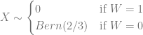
and 
We find that in scenario 1, 

In fact, as this table shows, the probabilities for all combinations of

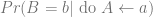
Now, consider the intervention of setting 

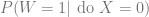


This is an example of why correlations are not causations: while the conditional probabilities 

Causal Probabilities
Suppose we know the causal graph, but not the individual probabilities. Let’s focus on scenario 1, where exercise causes overweight and heart disease. That is, the causal relation is as follows:

Looking at the table above, we see that the unconditional probability 

The reason is for this gap is that there is a counfounding variable, namely
Definition: 


To fix the effect of a confounder, we condition on

where
Contrast this with the formula for computing the conditional probability which is

Using the deconfounding formula (★) requires (a) knowing the causal graph, and (b) observing the confounders. If we get this wrong and control for the wrong confounders we can get the causal probabilities wrong, as demonstrated by the following example.
One way to describe causality theory is that it aims to clarify the situations under which correlation does in fact equal causation (i.e., the conditional probabilities are equal to the causal probabilities), and how (by appropriately controlling for confounders) we can get to such a situation.
Example (two diseases) Consider the diagram below where there are two diseases 


If you control for 


This relates to the joke “the probability of having 2 bombs on a plane is very low, so if I bring a bomb then it is very unlikely that there will be another bomb.”
In general, the causal graph can look as one of the following shapes:

If
Backdoor paths: If

We can show the following theorem:
Theorem: If there is no backdoor path then

Here is a “proof by picture”:

If there isn’t a backdoor path, we sort the graph in topological order, so that all the events that happen before 
Experimental Design
When we design experiments, we often want to estimate causal effects, and to do so we try to make sure we eliminate backdoor paths. Consider the example of a COVID vaccine trial. We let 


To fix this we can cut the backdoor path using a placebo: it cuts the backward path by removing the confounding variable of participation, since it ensure that (conditioning on 


Conditioning
In general, how does conditioning on some variable 
Average Treatment Effect and Propensity Score
Suppose we have some treatment variable 


The propensity score, defined as 

The proof is obtained by expanding out the claim, see below

Intuitively, knowing the probability that different groups of people get treatment allows us to make 
Calculating treatment effect using ML. Suppose that the treatment effect is 


Since both 

Instrumental Variables
When we cannot observe the counfounding variable, we can still sometimes use instrumental variables to estimate a causal effect.

Assume a linear model 


which is the ratio between two observable quantities.
Fairness
We focus on fairness in classification problems, rather than fairness in learning generative models or representation (which also have their own issues, see in particular this paper by Bender, Gebru, McMillan-Major, and “Shmitchell”).
In the public image, AI has been perceived to be very successful for some tasks, and some people might hope that it is more “objective” or “impartial” than human decisions which are known to be fraught with bias). However, there are some works suggesting this might not be the case:
- Usage in prediciting recidivism for bail decisions. For example in ProPublica Angwin, Larson, Mattu, and Kirchner showed that 44.9% of African Americans who didn’t reoffend were labeled higher risk, whereas only 23.5% of white defendants who didn’t reoffend were labeled as such.
- Machine vision can sometimes work better on some segments of population than others. For example, Buolamwini and Gebrue showed that some “gender classifiers” achieve 99.7% accuracy on white men but only 65.3% accuracy (not much better than coin toss) on black women.
- Lum and Isaac gave an example of a “positive feedback loop” in predictive policing in Oakland, CA. While drug use is fairly uniform across the city, the arrests are centered on particular neighborhood (that have more minority residents). In predictive policing, more police would be sent out to the places where arrests occured, hence only exercabating this disparate treatment.
Drug use in Oakland: 
Drug arrests in Oakland:

While algorithms can sometimes also help, the populations they help might not be distributed equally. For example, see this table from Gates, Perry and Zorn. A more accurate underwriting model (that can better predict the default probability) enables a lender to use a more agressive risk cut off and so end up lending to more people.

However, this is true within each subpopulation too, so it may be that if the model is less accurate in a certain subpopulation, then a profit-maximizing lender will unfairly offer fewer loans to this subpopulation.
Formalizing Unfairness
In the case of employment discrimination in the U.S., we have the following components:
- Protected class
- categories such as race, sex, nationality, citizenship, veteran status, etc.
- An unfairness metric, measuring either:
- disparate treatment
- disparate impact.
Employers are not allowed to discriminate across protected classes when hiring. The unfairness metric gives us a way to measure if there is discrimination with respected to a protected class. In particular, disparate impacts across different protected classes is often necessary but not sufficient evidence of discrimination.
Algorithms for Fairness: an Example
To see why algorithms, which at first glance seem agnostic to group membership, may exhibit disparate treatment or impact, we consider the following Google visualization by Wattenberg, Viégas, and Hardt.
Consider a blue population and an orange population for which there is no difference in the probability of a member of either population paying back the loan, but for which our model has different accuracies—in particular, the model is more accurate on the orange population. This is described by the plot below, in which the scores correspond to the model’s prediction of the probability of paying back the loan and opaque circles correspond to those who actually do not pay back the loan, whereas filled in circles correspond to those who do.

Suppose we are in charge of making a lending decision given the model prediction. A scenario in which we give everyone a loan would be fair, but would be bad us —we would go bankrupt!
Profit when giving everyone a loan:

If we wanted to maximize profit, we would, however, give more loans to the orange population (since we’re more sure about which members of the orange population would actually pay back their loans) by setting a lower threshold (in terms of the score given by our algorithm) above which we give out loans.

This maximizes profit but is blatantly unfair. We are treating the identical blue and orange groups differently, just because our model is more accurate on one than the other, and we also have disparate impact on the two groups. A non-defaulting applicant would be 78% likely to get a loan if they are a member of the orange group, but only 60% likely to get a loan if they are a member of the orange group.
This “profit maximization” is likely the end result of any sufficiently complex lending algorithm in the absence of a fairness intervention. Even if the algorithm does not explicitly rely on the group membership attribute, by simply optimizing it to maximize profit, it may well pick up on attributes that are correlated with group membership.
Suppose on the other hand that we wanted to mandate “equal treatment” in the sense of keeping the same thresholds for the blue and orange group. The result would be the following:

In this case, since the threshold are identical, the algorithm will be calibrated. 79% of the decisions we make will be the correct ones, for both the blue and orange population. So, from our point of view, the algorithm is fair and treats the blue and orange populations identically. However, from the point of view of the applicants, this is not the case. If you are a blue applicant that will pay your loan, you have 81% chance of getting a loan, but if you are an orange customer you only have 60% of getting it. This demonstrates that defining fairness is quite delicate. In particular the above “color blind” algorithm is still arguable unfair.
This difference between the point of view of the lender and lendee also arose in the recidivism case mentioned above. From the point of view of the defendant that would not recidivate, the algorithm was more likely to label them as “high risk” if they were Black than if they were white. From the point of view of the decision maker, the algorithm was calibrated, and if anything it was a bit more likely that a white defendant labeled high risk would not recidivate than a Black defendant. See (slightly rounded and simplified) data below

If we wanted to achieve demographic parity (both populations get same total number of loans) or equal opportunity (true positive rate same for both) then we can do so, but again using different thresholds for each group:


Fico Scores and Different Types of Fairness
While the above was a hypothetical scenario, a real life example was shown by Hardt, Price and Srebro using credit (also known as FICO) scores, as described by the plot below:

For a single threshold, around 75% of Asian candidates will get loans, whereas only around 20% of Black candidates will get loans. To ensure that all groups get loans at the same rate, we would need to set the thresholds differently. In order to equalize opportunity, we’d also need to initialize the thresholds differently as well.
We see that we have different notions of what it means to be fair and that each of these different notions result in different algorithms.
Fairness and Causality
Berkeley graduate admissions in 1973 had the following statistics:
- 44% male applicants admitted, 35% female applicants admitted;
- However, female acceptance rate was higher at the department level, for most departments.

This paradox is commonly referred to as Simpson’s Paradox.
A “fair” causal model for this scenario might be as follows:

In the above, perhaps gender has a causal impact on the choice of department to which the applicant applies. However, a fair application process would, conditional on the department, be independent of gender of the applicant.
However, not all models that follow this causal structure are necessarily fair. In the case Griggs v. Duke Power Co., 1971, the court ruled that decision-making under the following causal model was unfair:

While the model appears to be fair, since the job offer is conditionall independent of race, given the diploma, the court ruled that the job did not actually require a high school diploma. Hence, using the diploma as a factor in hiring decisions was really just a proxy for race, resulting in essentially purposeful unfair discrimination based on race. This creation of proxies is referred to as redlining.
Bottom Line
We cannot come up with universal fairness criteria. The notion of fairness itself is based on assumptions about:
- representation of data
- relationships to unmeasured inputs and outcomes
- causal relation of inputs, predictions, outcomes.
Fairness depends on what we choose to measure to observe, in both inputs and outputs, and how we choose to act upon them. In particular, we have the following causal structure, wherein measure inputs, decision-making, and measured outcomes all play a role in affecting the real-world and function together in a feedback cycle:

A more comprehensive illustration is given in this paper of Friedler, Scheidegger, and Venkatasubramanian:
