Guest post by Greg Kuperberg: Archimedes’ other principle and quantum supremacy

Scott’s Introduction: Happy Thanksgiving! Please join me in giving thanks for the beautiful post below, by friend-of-the-blog Greg Kuperberg, which tells a mathematical story that stretches from the 200s BC all the way to Google’s quantum supremacy result last month.

Archimedes’ other principle and quantum supremacy

by Greg Kuperberg

Note: UC Davis is hiring in CS theory! Scott offered me free ad space if I wrote a guest post, so here we are. The position is in all areas of CS theory, including QC theory although the search is not limited to that.

In this post, I wear the hat of a pure mathematician in a box provided by Archimedes. I thus set aside what everyone else thinks is important about Google’s 53-qubit quantum supremacy experiment, that it is a dramatic milestone in quantum computing technology. That’s only news about the physical world, whose significance pales in comparison to the Platonic world of mathematical objects. In my happy world, I like quantum supremacy as a demonstration of a beautiful coincidence in mathematics that has been known for more than 2000 years in a special case. The single-qubit case was discovered by Archimedes, duh. As Scott mentions in Quantum Computing Since Democritus, Bill Wootters stated the general result in a 1990 paper, but Wootters credits a 1974 paper by the Czech physicist Stanislav Sýkora. I learned of it in the substantially more general context of symplectic geometric that mathematicians developed independently between Sýkora’s prescient paper and Wootters’ more widely known citation. Much as I would like to clobber you with highly abstract mathematics, I will wait for some other time.

Suppose that you pick a pure state \(|\psi\rangle\) in the Hilbert space \(\mathbb{C}^d\) of a \(d\)-dimensional qudit, and then make many copies and fully measure each one, so that you sample many times from some distribution \(\mu\) on the \(d\) outcomes. You can think of such a distribution \(\mu\) as a classical randomized state on a digit of size \(d\). The set of all randomized states on a \(d\)-digit makes a \((d-1)\)-dimensional simplex \(\Delta^{d-1}\) in the orthant \(\mathbb{R}_{\ge 0}^d\). The coincidence is that if \(|\psi\rangle\) is uniformly random in the unit sphere in \(\mathbb{C}^d\), then \(\mu\) is uniformly random in \(\Delta^{d-1}\). I will call it the Copenhagen map, since it expresses the Copenhagen interpretation of quantum mechanics that amplitudes yield probabilities. Here is a diagram of the Copenhagen map of a qutrit, except with the laughable simplification of the 5-sphere in \(\mathbb{C}^3\) drawn as a 2-sphere.

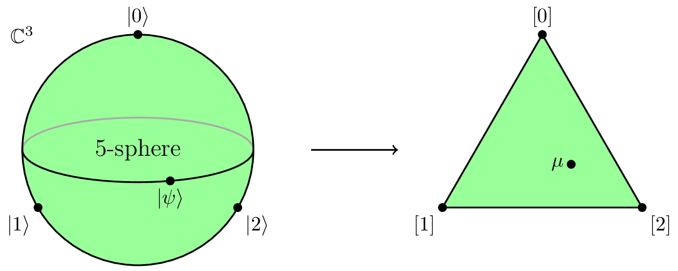
If you pretend to be a bad probability student, then you might not be surprised by this coincidence, because you might suppose that all probability distributions are uniform other than treacherous exceptions to your intuition. However, the principle is certainly not true for a “rebit” (a qubit with real amplitudes) or for higher-dimensional “redits.” With real amplitudes, the probability density goes to infinity at the sides of the simplex \(\Delta^{d-1}\) and is even more favored at the corners. It also doesn’t work for mixed qudit states; the projection then favors the middle of \(\Delta^{d-1}\).

Archimedes’ theorem

The theorem of Archimedes is that a natural projection from the unit sphere to a circumscribing vertical cylinder preserves area. The projection is the second one that you might think of: Project radially from a vertical axis rather than radially in all three directions. Since Archimedes was a remarkably prescient mathematician, he was looking ahead to the Bloch sphere of pure qubit states \(|\psi\rangle\langle\psi|\) written in density operator form. If you measure \(|\psi\rangle\langle\psi|\) in the computational basis, you get a randomized bit state \(\mu\) somewhere on the interval from guaranteed 0 to guaranteed 1.

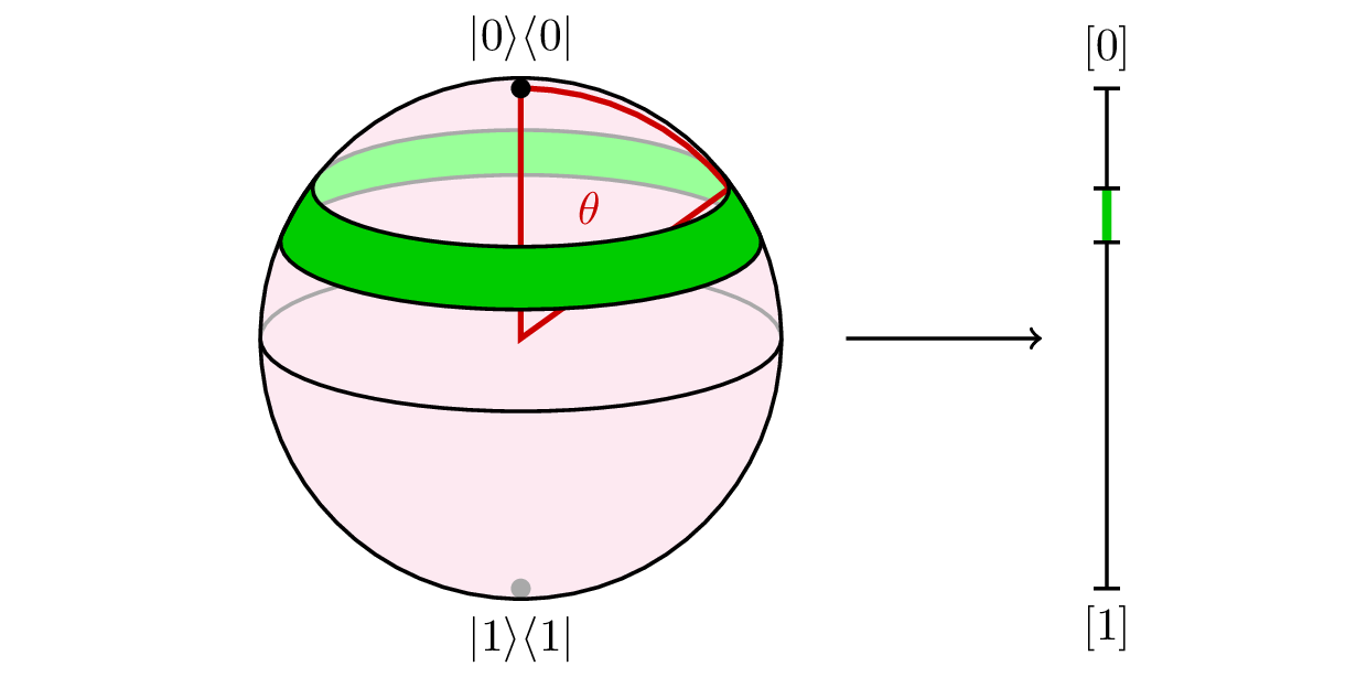
This transformation from a quantum state to a classical randomized state is a linear projection to a vertical axis. It is the same as Archimedes’ projection, except without the angle information. It doesn’t preserve dimension, but it does preserve measure (area or length, whatever) up to a factor of \(2\pi\). In particular, it takes a uniformly random \(|\psi\rangle\langle\psi|\) to a uniformly random \(\mu\).

Archimedes’ projection is also known as the Lambert cylindrical map of the world. This is the map that squishes Greenland along with the top of North America and Eurasia to give them proportionate area.

(I forgive Lambert if he didn’t give prior credit to Archimedes. There was no Internet back then to easily find out who did what first.) Here is a calculus-based proof of Archimedes’ theorem: In spherical coordinates, imagine an annular strip on the sphere at a polar angle of \(\theta\). (The polar angle is the angle from vertical in spherical coordinates, as depicted in red in the Bloch sphere diagram.) The strip has a radius of \(\sin\theta\), which makes it shorter than its unit radius friend on the cylinder. But it’s also tilted from vertical by an angle of \(\frac{\pi}2-\theta\), which makes it wider by a factor of \(1/(\sin \theta)\) than the height of its projection onto the \(z\) axis. The two factors exactly cancel out, making the area of the strip exactly proportional to the length of its projection onto the \(z\) axis. This is a coincidence which is special to the 2-sphere in 3 dimensions. As a corollary, we get that the surface area of a unit sphere is \(4\pi\), the same as an open cylinder with radius 1 and height 2. If you want to step through this in even more detail, Scott mentioned to me an action video which is vastly spiffier than anything that I could ever make.

The projection of the Bloch sphere onto an interval also shows what goes wrong if you try this with a rebit. The pure rebit states — again expressed in density operator form \(|\psi\rangle\langle\psi|\) are a great circle in the Bloch sphere. If you linearly project a circle onto an interval, then the length of the circle is clearly bunched up at the ends of the interval and the projected measure on the interval is not uniform.

Sýkora’s generalization

It is a neat coincidence that the Copenhagen map of a qubit preserves measure, but a proof that relies on Archimedes’ theorem seems to depend on the special geometry of the Bloch sphere of a qubit. That the higher-dimensional Copenhagen map also preserves measure is downright eerie. Scott challenged me to write an intuitive explanation. I remembered two different (but similar) proofs, neither of which is original to me. Scott and I disagree as to which proof is nicer.

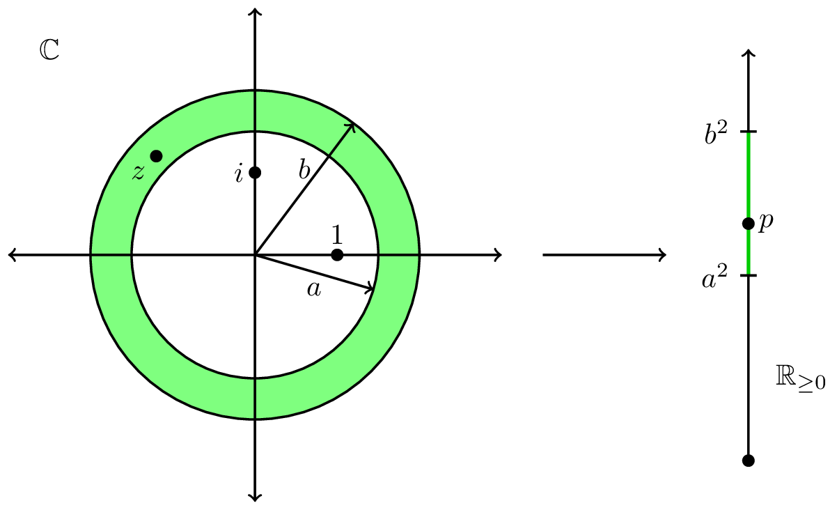
As a first step of the first proof, it is easy to show that the Copenhagen map \(p = |z|^2\) for a single amplitude \(z\) preserves measure as a function from the complex plane \(\mathbb{C}\) to the ray \(\mathbb{R}_{\ge 0}\). The region in the complex numbers \(\mathbb{C}\) where the length of \(z\) is between \(a\) and \(b\), or \(a \le |z| \le b\), is \(\pi(b^2 – a^2)\). The corresponding interval for the probability is \(a^2 \le p \le b^2\), which thus has length \(b^2-a^2\). That’s all, we’ve proved it! More precisely, the area of any circularly symmetric region in \(\mathbb{C}\) is \(\pi\) times the length of its projection onto \(\mathbb{R}_{\ge 0}\).

The second step is to show the same thing for the Copenhagen map from the \(d\)-qudit Hilbert space \(\mathbb{C}^d\) to the \(d\)-digit orthant \(\mathbb{R}_{\ge 0}^d\), again without unit normalization. It’s also measure-preserving, up to a factor of \(\pi^d\) this time, because it’s the same thing in each coordinate separately. To be precise, the volume ratio holds for any region in \(\mathbb{C}^d\) that is invariant under separately rotating each of the \(d\) phases. (Because you can approximate any such region with a union of products of thin annuli.)

The third and final step is the paint principle for comparing surface areas. If you paint the hoods of two cars with the same thin layer of paint and you used the same volume of paint for each one, then you can conclude that the two car hoods have nearly same area. In our case, the Copenhagen map takes the region \[ 1 \le |z_0|^2 + |z_1|^2 + \cdots + |z_{d-1}|^2 \le 1+\epsilon \] in \(\mathbb{C}^d\) to the region \[ 1 \le p_0 + p_1 + \cdots + p_{d-1} \le 1+\epsilon \] in the orthant \(\mathbb{R}_{\ge 0}^d\). The former is the unit sphere \(S^{2d-1}\) in \(\mathbb{C}^d\) painted to a thickness of roughly \(\epsilon/2\). The latter is the probability simplex \(\Delta^{n-1}\) painted to a thickness of exactly \(\epsilon\). Taking the limit \(\epsilon \to 0\), the Copenhagen map from \(S^{2d-1}\) to \(\Delta^{n-1}\) preserves measure up to a factor of \(2\pi^n\).

You might wonder “why” this argument works even if you accept that it does work. The key is that the exponent 2 appears in two different ways: as the dimension of the complex numbers, and as the exponent used to set probabilities and define spheres. If we try the same argument with real amplitudes, then the volume between “spheres” of radius \(a\) and \(b\) is just \(2(b-a)\), which does not match the length \(b^2-a^2\). The Copenhagen map for a single real amplitude is the parabola \(p = x^2\), which clearly distorts length since it is not linear. The higher-dimensional real Copenhagen map similarly distorts volumes, whether or not you restrict to unit-length states.

If you’re a bitter-ender who still wants Archimedes’ theorem for real amplitudes, then you might consider the variant formula \(p = |x|\) to obtain a probability \(p\) from a “quantum amplitude” \(x\). Then the “Copenhagen” map does preserve measure, but for the trivial reason that \(x = \pm p\) is not really a quantum amplitude, it is a probability with a vestigial sign. Also the unit “sphere” in \(\mathbb{R}^d\) is not really a sphere in this theory, it is a hyperoctahedron. The only “unitary” operators that preserve the unit hyperoctahedron are signed permutation matrices. You can only use them for reversible classical computing or symbolic dynamics; they don’t have the strength of true quantum computing or quantum mechanics.

The fact that the Copenhagen map preserves measure also yields a bonus calculation of the volume of the unit ball in \(2d\) real dimensions, if we interpret that as \(d\) complex dimensions. The ball \[ |z_0|^2 + |z_1|^2 + \cdots + |z_{d-1}|^2 \le 1 \] in \(\mathbb{C}^d\) is sent to a different simplex \[ p_0 + p_1 + \cdots + p_{d-1} \le 1 \] in \(\mathbb{R}_{\ge 0}^d\). If we recall that the volume of a \(d\)-dimensional pyramid is \(\frac1d\) times base times height and calculate by induction on \(d\), we get that this simplex has volume \(\frac1{d!}\). Thus, the volume of the \(2d\)-dimensional unit ball is \(\frac{\pi^d}{d!}\).

You might ask whether the volume of a \(d\)-dimensional unit ball is always \(\frac{\pi^{d/2}}{(d/2)!}\) for both \(d\) even and odd. The answer is yes if we interpret factorials using the gamma function formula \(x! = \Gamma(x+1)\) and look up that \(\frac12! = \Gamma(\frac32) = \frac{\sqrt{\pi}}2\). The gamma function was discovered by Euler as a solution to the question of defining fractional factorials, but the notation \(\Gamma(x)\) and the cumbersome shift by 1 is due to Legendre. Although Wikipedia says that no one knows why Legendre defined it this way, I wonder if his goal was to do what the Catholic church later did for itself in 1978: It put a Pole at the origin.

(Scott wanted to censor this joke. In response, I express my loyalty to my nation of birth by quoting the opening of the Polish national anthem: “Poland has not yet died, so long as we still live!” I thought at first that Stanislav Sýkora is Polish since Stanisław and Sikora are both common Polish names, but his name has Czech spelling and he is Czech. Well, the Czechs are cool too.)

Sýkora’s 1974 proof of the generalized Archimedes’ theorem is different from this one. He calculates multivariate moments of the space of unit states \(S^{2d-1} \subseteq \mathbb{C}^d\), and confirms that they match the moments in the probability simplex \(\Delta^{d-1}\). There are inevitably various proofs of this result, and I will give another one.

Another proof, and quantum supremacy

There is a well-known and very useful algorithm to generate a random point on the unit sphere in either \(\mathbb{R}^d\) or \(\mathbb{C}^d\), and a similar algorithm to generate a random point in a simplex. In the former algorithm, we make each real coordinate \(x\) into an independent Gaussian random variable with density proportional to \(e^{-x^2}\;dx\), and then rescale the result to unit length. Since the exponents combine as \[ e^{-x_0^2}e^{-x_1^2}\cdots e^{-x_{d-1}^2} = e^{-(x_0^2 + x_1^2 + \cdots + x_{d-1}^2)}, \] we learn that the total exponent is spherically symmetric. Therefore after rescaling, the result is a uniformly random point on the unit sphere \(S^{d-1} \subseteq \mathbb{R}^d\). Similarly, the other algorithm generates a point in the orthant \(\mathbb{R}_{\ge 0}^d\) by making each real coordinate \(p \ge 0\) an independent random variable with exponential distribution \(e^{-p}\;dp\). This time we rescale the vector until its sum is 1. This algorithm likewise produces a uniformly random point in the simplex \(\Delta^{d-1} \subseteq \mathbb{R}_{\ge 0}^d\) because the total exponent of the product \[ e^{-p_0}e^{-p_1}\cdots e^{-p_{d-1}} = e^{-(p_0 + p_1 + \cdots + p_{d-1})} \] only depends on the sum of the coordinates. Wootters describes both of these algorithms in his 1990 paper, but instead of relating them to give his own proof of the generalized Archimedes’ theorem, he cites Sýkora.

The gist of the proof is that the Copenhagen map takes the Gaussian algorithm to the exponential algorithm. Explicitly, the Gaussian probability density for a single complex amplitude \[ z = x+iy = re^{i\theta} \] can be converted from Cartesian to polar coordinate as follows: \[ \frac{e^{-|z|^2}\;dx\;dy}{\pi} = \frac{e^{-r^2}r\;dr\;d\theta}{\pi}. \] I have included the factor of \(r\) that is naturally present in an area integral in polar coordinates. We will need it, and it is another way to see that the theorem relies on the fact that the complex numbers are two-dimensional. To complete the proof, we substitute \(p = r^2\) and remember that \(dp = 2r\;dr\), and then integrate over \(\theta\) (trivially, since the integrand does not depend on \(\theta\)). The density simplifies to \(e^{-p}\;dp\), which is exactly the exponential distribution for a real variable \(p \ge 0\). Since the Copenhagen map takes the Gaussian algorithm to the exponential algorithm, and since each algorithm produces a uniformly random point, the Copenhagen map must preserve uniform measure. (Scott likes this proof better because it is algorithmic, and because it is probabilistic.)

Now about quantum supremacy. You might think that a random chosen quantum circuit on \(n\) qubits produces a nearly uniformly random quantum state \(|\psi\rangle\) in their joint Hilbert space, but it’s not quite not that simple. When \(n=53\), or otherwise as \(n \to \infty\), a manageable random circuit is not nearly creative enough to either reach or approximate most of the unit states in the colossal Hilbert space of dimension \(d = 2^n\). The state \(|\psi\rangle\) that you get from (say) a polynomial-sized circuit resembles a fully random state in various statistical and computational respects, both proven and conjectured. As a result, if you measure the qubits in the computational basis, you get a randomized state on \(n\) bits that resembles a uniformly random point in \(\Delta^{2^n-1}\).

If you choose \(d\) probabilities, and if each one is an independent exponential random variable, then the law of large numbers says that the sum (which you use for rescaling) is close to \(d\) when \(d\) is large. When \(d\) is really big like \(2^{53}\), a histogram of the probabilities of the bit strings of a supremacy experiment looks like an exponential curve \(f(p) \propto e^{-pd}\). In a sense, the statistical distribution of the bit strings is almost the same almost every time, independent of which random quantum circuit you choose to generate them. The catch is that the position of any given bit string does depend on the circuit and is highly scrambled. I picture it in my mind like this:

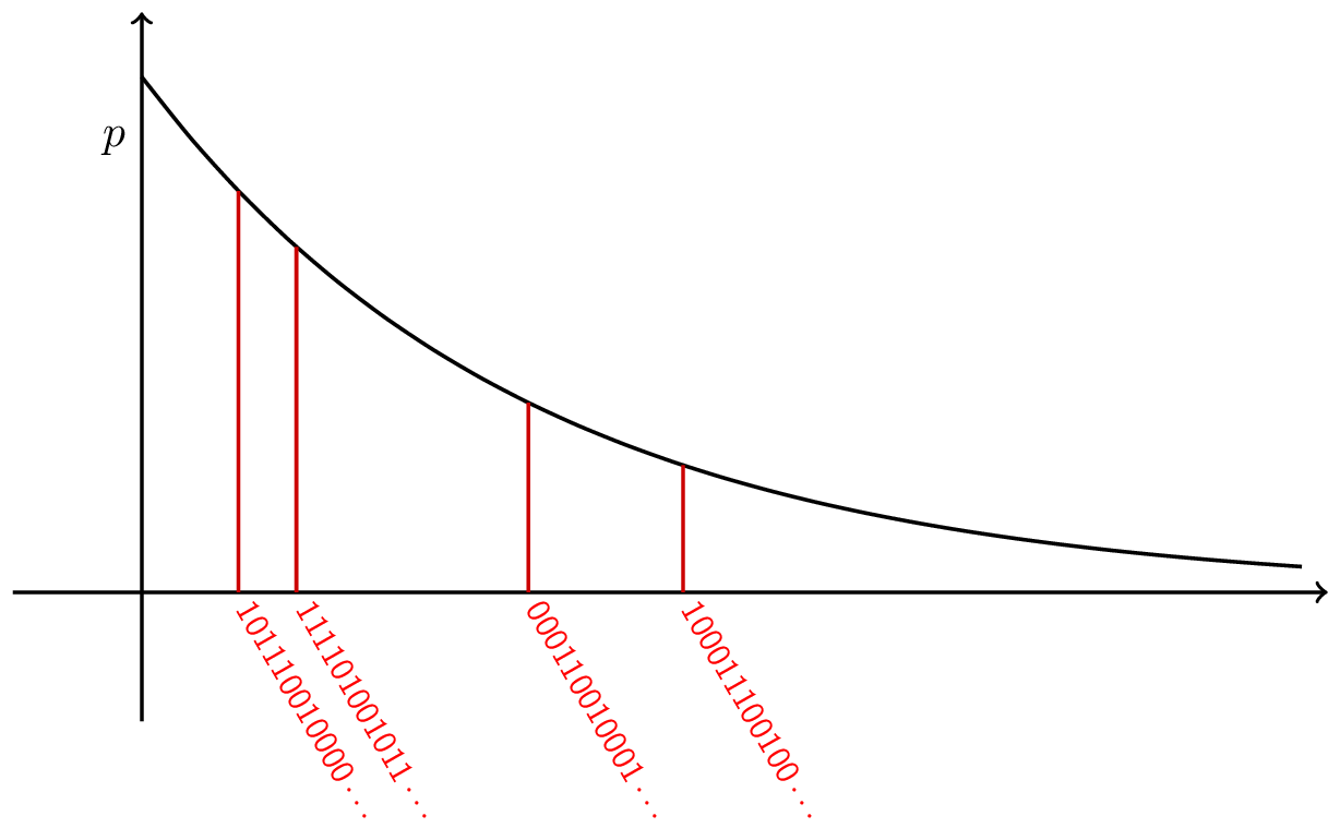
It is thought to be computationally intractable to calculate where each bit string lands on this exponential curve, or even where just one of them does. (The exponential curve is attenuated by noise in the actual experiment, but it’s the same principle.) That is one reason that random quantum circuits are supreme.