Mathematics of the impossible, Chapter 9, Log-depth circuits

Thoughts 2023-04-19

In this chapter we investigate circuits of logarithmic depth. Again, several surprises lay ahead, including a solution to the teaser in Chapter 1!

Let us begin slowly with some basic properties of these circuits so as to get familiar with them. The next exercise shows that circuits of depth $d\log n$ for a constant $d$ also have power size, so we don’t need to bound the size separately.

Exercise 9.1. A circuit of depth $d$ has size $\le c^{d}$ without loss of generality.

The next exercises shows how to compute several simple functions by log-depth circuits.

Exercise 9.2. Prove that the Or, And, and Parity functions on $n$ bits have circuits of depth $c\log n$ .

Prove that any $f: \{0,1\}^n \to \{0,1\}$ computable by an AltCkt of depth $d$ and size $s\ge n$ is also computable by a circuit of depth $cd\log s$ and size $s^{c}$ .

Next, let us relate these circuits to branching programs. The upshot is that circuits of logarithmic depth are a special case of power-size branching programs, and the latter are a special case of circuits of log-square depth.

Theorem 9.1. Directed reachability has circuits of depth $c\log ^{2}n$ and size $n^{c}$ . In particular, the same holds for any function in NL, and any function with power-size branching programs.

Proof. On input a graph $G$ on $u$ nodes and two nodes $s$ and $t$ , let $M$ be the $u\times u$ transition matrix corresponding to $G$ , where $M_{i,j}=1$ iff edge $j\to i$ is in $G$ .

Transition matrices are multiplied as normal matrices, except that “ $+$ ” is replaced with “ $\vee$ ,” which suffices to know connectivity. To answer directed reachability we compute entry $t$ of $M^{u}v$ , where $v$ has a $1$ corresponding to $s$ and $0$ everywhere else. (We can modify the graph to add a self-loop on node $t$ so that we can reach $t$ in exactly $u$ steps iff we reach $t$ in any number of steps.)

Computing $M^{u}$ can be done by squaring $c\log u$ times $M$ . Each squaring can be done in depth $c\log u$ , by Exercise 9.2. This establishes the first claim, since $u\le n$ .

The “in particular” follows because those functions can be reduced to directed reachability efficiently. QED

Conversely, we have the following.

Theorem 9.2. Any function $f: \{0,1\}^n \to \{0,1\}$ computed by a circuit of depth $d$ can be computed by a branching program of size $2^{d}$ .

In particular, functions computed by circuits of logarithmic depth can be computed by branching programs of power size.

Later in this chapter we will prove a stronger and much less obvious result.

Proof. We proceed by induction on the depth of the circuit $C$ . If the depth is $1$ then $C$ is either a constant or an input bit, and a branching program of size $1$ is available by definition.

Suppose the circuit $C$ has the form $C_{1}\wedge C_{2}$ . By induction, $C_{1}$ and $C_{2}$ have branching programs $B_{1}$ and $B_{2}$ each of size $2^{d-1}$ . A branching program $B$ for $C$ of size $2^{d}$ is obtained by rewiring the edges leading to states labelled $1$ in $B_{1}$ to the start state of $B_{2}$ . The start state of $B$ is the start state of $B_{1}$ . QED

Exercise 9.3. Finish the proof by analyzing the case $C=C_{1}\vee C_{2}$ .

Definition 9.1. $\text {NC}^{i}$ is the class of functions $f:\{0,1\}^* \to \{0,1\}^*$ computable by circuits that have depth $a\log ^{i}n$ and size $n^{a}$ , for some constant $a$ . The circuits are uniform if they can be computed in $\text {L}$ .

The class $\text {NC}^{0}$ is also of great interest. It can be more simply defined as the class of functions where each output bit depends on a constant number of input bits. We will see many surprising useful things that can be computed in this class.

The previous results give, for uniform circuits:

$\begin{aligned} \text {NC}^{0}\subseteq \text {\ensuremath {\text {NC}^{1}\subseteq }}\text {L}\subseteq \text {NL}\subseteq \text {NC}^{2}\subseteq \text {NC}^{3}\subseteq \cdots \subseteq \text {P}. \end{aligned}$

The only inclusion known to be strict is the first one:

Exercise 9.4. Prove that $\text {NC}^{0}\ne \text {NC}^{1}$ . (Mostly to practice definitions.)

9.1 The power of $\text {NC}^{1}$ : Arithmetic

In this section we illustrate the power of $\text {NC}^{1}$ by showing that the same basic arithmetic which we saw is doable in $\text {L}$ (Theorem 7.5) can in fact be done in $\text {NC}^{1}$ as well.

Theorem 9.3. The following problems are in NC $^{1}$ :

Addition of two input integers.
Iterated addition: Addition of any number of input integers.
Multiplication of two input integers.
Iterated multiplication: Multiplication of any number of input integers.
Division of two integers.

Exercise 9.5. Prove Item 1. in Theorem 9.3.

Iterated addition is surprisingly non-trivial. We can’t use the methods from the proof of Theorem 7.5. Instead, we rely on a new and very clever technique.

Proof of Item 2. in Theorem 9.3.. We use “2-out-of-3:” Given 3 integers $X,Y,Z$ , we compute 2 integers $A,B$ such that

$\begin{aligned} X+Y+Z=A+B, \end{aligned}$

where each bit of $A$ and $B$ only depends on three bits, one from $X$ , one from $Y$ , and one from $Z$ . Thus $A$ and $B$ can be computed in NC $^{0}$ .

If we can do this, then to compute iterated addition we construct a tree of logarithmic depth to reduce the original sum to a sum $2$ terms, which we add as in Item 1.

Here’s how it works. Note $X_{i}+Y_{i}+Z_{i}\leq 3$ . We let $A_{i}$ be the least significant bit of this sum, and $B_{i+1}$ the most significant one. Note that $A_{i}$ is the XOR $X_{i}+Y_{i}+Z_{i}$ , while $B_{i+1}$ is the majority of $X_{i},Y_{i},Z_{i}$ . QED

The following corollary will also be used to solve the teaser in Chapter 1.

Corollary 9.1. Majority is in $\text {NC}^{1}$ .

Exercise 9.6. Prove it.

Exercise 9.7. Prove Item 3. in Theorem 9.3.

Next we turn to iterated multiplication. The idea is to follow the proof for L in section 7.2.1. We shall use CRR again. The problem is that we still had to perform iterated multiplication, albeit only in $\mathbb {Z}_{p}$ for $p\le n^{c}$ . One more mathematical result is useful now:

Theorem 9.4. If $p$ is a prime then $(\mathbb {Z}_{p}-\{0\})$ is a cyclic group, meaning that there exists a generator $g\in (\mathbb {Z}_{p}-\{0\}):\forall x\in (\mathbb {Z}_{p}-\{0\}),x=g^{i}$ , for some $i\in \mathbb {Z}$ .

Example 9.1. For $p=5$ we can take $g=2$ : $2^{0}=1,2^{1}=2,2^{2}=4,2^{3}=8=3$ .

Proof of Item 4. in Theorem 9.3. We follow the proof for L in section 7.2.1. To compute iterated product of integers $r_{1},r_{2},\ldots ,r_{t}$ modulo $p$ , use Theorem 9.4 to compute exponents $e_{1},e_{2},\ldots ,e_{t}$ s.t.

$\begin{aligned} r_{i}=g^{e_{i}}. \end{aligned}$

Then $\prod _{i}r_{i}\mod p=g^{\sum _{i}e_{i}}$ . We can use Item 2. to compute the iterated addition of the exponents. Note that computing the exponent of a number mod $p$ , and vice versa, can be done in log-depth since the numbers have $c\log n$ bits (as follows for example by combining Theorem 2.3 and Exercise 9.2). QED

One can also compute division, and make all these circuits uniform, but we won’t prove this now.

9.2 Computing with 3 bits of memory

We now move to a surprising result that in particular strengthens Theorem 9.2. For a moment, let’s forget about circuits, branching programs, etc. and instead consider a new, minimalistic type of programs. We will have 3 one-bit registers: $R_{0},R_{1},R_{2}$ , operating modulo $2$ . We allow the following operations

$\begin{aligned} R_{i} & +=R_{j},\\ R_{i} & +=R_{j}x_{k} \end{aligned}$

where $x_{k}$ is an input bit, for any $i,j\in \{0,1,2\}$ , with $i\ne j$ . (Talk about RISC!) Here $R_{i}+=R_{j}$ means to add the content of $R_{j}$ to $R_{i}$ , while $R_{i}+=R_{j}x_{k}$ means to add $R_{j}x_{k}$ to $R_{i}$ , where $R_{j}x_{k}$ is the product (a.k.a. And) of $R_{j}$ and $x_{k}$ .

Definition 9.2. For $i,j$ and $f: \{0,1\}^n \to \{0,1\}$ we say that a program is for (or equivalent to)

$\begin{aligned} R_{i}+=R_{j}f \end{aligned}$

if for every input $x$ and initial values of the registers, executing the program is equivalent to the instruction $R_{i}+=R_{j}f(x)$ , where note that $R_{j}$ and $R_{k}$ are unchanged.

Also note that if we repeat twice a program for $R_{i}+=R_{j}f$ then no register changes (recall the sum is modulo $2$ , so $1+1=0$ ). This feature is critically exploited later to “clean up” computation.

We now state and prove the surprising result. It is convenient to state it for circuits with Xor instead of Or gates. This is without loss of generality since $x\vee y=x+y+x\wedge y$ .

Theorem 9.5. [44, 15] Suppose $f: \{0,1\}^n \to \{0,1\}$ is computable by circuits of depth $d$ with Xor and And gates. For every $i\ne j$ there is a program of length $\le c4^{d}$ for

$\begin{aligned} R_{i} & +=R_{j}f. \end{aligned}$

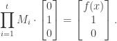
Once such a program is available, we can start with register values $(0,1,0)$ and $i=0,j=1$ to obtain $f(x)$ in $R_{0}$ .

Proof. We proceed by induction on $d$ . When $d=1$ the circuit is simply outputting a constant or one of the input bits, which we can compute with the corresponding instructions. (If the circuit is the constant zero then the empty program would do.)

Proceeding with the induction step:

A program for $R_{i}+=R_{j}(f_{1}+f_{2})$ is simply given by the concatenation of (the programs for)

$\begin{aligned} R_{i} & +=R_{j}f_{1}\\ R_{i} & +=R_{j}f_{2}. \end{aligned}$

Less obviously, a program for $R_{i}+=R_{j}(f_{1}\wedge f_{2})$ is given by

$\begin{aligned} R_{i} & +=R_{k}f_{1}\\ R_{k} & +=R_{j}f_{2}\\ R_{i} & +=R_{k}f_{1}\\ R_{k} & +=R_{j}f_{2}. \end{aligned}$

QED

Exercise 9.8. Prove that the program for $f_{1}\wedge f_{2}$ in the proof works. Write down the contents of the registers after each instruction in the program.

A similar proof works over other fields as well.

We can now address the teaser Theorem 1.1 from Chapter 1.

Proof of Theorem 1.1.. Combine Corollary 9.1 with Theorem 9.5. QED

Corollary 9.2. Iterated product of 3×3 matrices over $\mathbb {F}_{2}$ is complete for NC $^{1}$ under projections.

That is, the problem is in NC $^{1}$ and for any $f\in \text {NC}^{1}$ and $n$ one can write a sequence of $t=n^{c}$ 3×3 matrices $M_{1},M_{2},\ldots ,M_{t}$ where each entry is either a constant or an input variable $x_{i}$ s.t. for every $x\in \{0,1\} ^{n}$ :

$\begin{aligned} \prod _{i=1}^{t}M_{i}\cdot \begin {bmatrix}0\\ 1\\ 0 \end {bmatrix}=\begin {bmatrix}f(x)\\ 1\\ 0 \end {bmatrix}. \end{aligned}$

Exercise 9.9. Prove this.

9.3 Linear-size log-depth

It is unknown whether NP has linear-size circuits of logarithmic depth! But there is a non-trivial simulation of such circuits by AltCkts of depth 3 of sub-exponential size.

Theorem 9.6. [67] Any circuit $C: \{0,1\}^n \to \{0,1\}$ of size $an$ and depth $a\log n$ has an equivalent alternating circuit of depth 3 and size $2^{c_{a}n/\log \log n}$ .

The idea is… yes! Once again, we are going to guess computation. It is possible to guess the values of about $n/\log \log n$ wires to reduce the depth to say $0.1\log n$ , and the rest is brute-forced. For an exposition, see [73].

Notes

Our presentation of Theorem 9.5 follows [18].

[1] Amir Abboud, Arturs Backurs, and Virginia Vassilevska Williams. Tight hardness results for LCS and other sequence similarity measures. In Venkatesan Guruswami, editor, IEEE 56th Annual Symposium on Foundations of Computer Science, FOCS 2015, Berkeley, CA, USA, 17-20 October, 2015, pages 59–78. IEEE Computer Society, 2015.

[2] Leonard Adleman. Two theorems on random polynomial time. In 19th IEEE Symp. on Foundations of Computer Science (FOCS), pages 75–83. 1978.

[3] Mikl�s Ajtai. $\Sigma \sp {1}\sb {1}$ -formulae on finite structures. Annals of Pure and Applied Logic, 24(1):1–48, 1983.

[4] Mikl�s Ajtai. A non-linear time lower bound for boolean branching programs. Theory of Computing, 1(1):149–176, 2005.

[5] Eric Allender. A note on the power of threshold circuits. In 30th Symposium on Foundations of Computer Science, pages 580–584, Research Triangle Park, North Carolina, 30 October–1 November 1989. IEEE.

[6] Eric Allender. The division breakthroughs. Bulletin of the EATCS, 74:61–77, 2001.

[7] Eric Allender and Michal Koucký. Amplifying lower bounds by means of self-reducibility. J. of the ACM, 57(3), 2010.

[8] Noga Alon, Oded Goldreich, Johan H�stad, and Ren� Peralta. Simple constructions of almost $k$ -wise independent random variables. Random Structures & Algorithms, 3(3):289–304, 1992.

[9] Dana Angluin and Leslie G. Valiant. Fast probabilistic algorithms for hamiltonian circuits and matchings. J. Comput. Syst. Sci., 18(2):155–193, 1979.

[10] Sanjeev Arora, Carsten Lund, Rajeev Motwani, Madhu Sudan, and Mario Szegedy. Proof verification and the hardness of approximation problems. J. of the ACM, 45(3):501–555, May 1998.

[11] Arturs Backurs and Piotr Indyk. Edit distance cannot be computed in strongly subquadratic time (unless SETH is false). SIAM J. Comput., 47(3):1087–1097, 2018.

[12] Kenneth E. Batcher. Sorting networks and their applications. In AFIPS Spring Joint Computing Conference, volume 32, pages 307–314, 1968.

[13] Paul Beame, Stephen A. Cook, and H. James Hoover. Log depth circuits for division and related problems. SIAM J. Comput., 15(4):994–1003, 1986.

[14] Paul Beame, Michael Saks, Xiaodong Sun, and Erik Vee. Time-space trade-off lower bounds for randomized computation of decision problems. J. of the ACM, 50(2):154–195, 2003.

[15] Michael Ben-Or and Richard Cleve. Computing algebraic formulas using a constant number of registers. SIAM J. on Computing, 21(1):54–58, 1992.

[16] Samuel R. Buss and Ryan Williams. Limits on alternation trading proofs for time-space lower bounds. Comput. Complex., 24(3):533–600, 2015.

[17] Lijie Chen and Roei Tell. Bootstrapping results for threshold circuits “just beyond” known lower bounds. In Moses Charikar and Edith Cohen, editors, Proceedings of the 51st Annual ACM SIGACT Symposium on Theory of Computing, STOC 2019, Phoenix, AZ, USA, June 23-26, 2019, pages 34–41. ACM, 2019.

[18] Richard Cleve. Towards optimal simulations of formulas by bounded-width programs. Computational Complexity, 1:91–105, 1991.

[19] Stephen A. Cook. A hierarchy for nondeterministic time complexity. J. of Computer and System Sciences, 7(4):343–353, 1973.

[20] L. Csanky. Fast parallel matrix inversion algorithms. SIAM J. Comput., 5(4):618–623, 1976.

[21] Lance Fortnow. Time-space tradeoffs for satisfiability. J. Comput. Syst. Sci., 60(2):337–353, 2000.

[22] Aviezri S. Fraenkel and David Lichtenstein. Computing a perfect strategy for n x n chess requires time exponential in n. J. Comb. Theory, Ser. A, 31(2):199–214, 1981.

[23] Michael L. Fredman and Michael E. Saks. The cell probe complexity of dynamic data structures. In ACM Symp. on the Theory of Computing (STOC), pages 345–354, 1989.

[24] Anka Gajentaan and Mark H. Overmars. On a class of ${O}(n^2)$ problems in computational geometry. Comput. Geom., 5:165–185, 1995.

[25] M. R. Garey and David S. Johnson. Computers and Intractability: A Guide to the Theory of NP-Completeness. W. H. Freeman, 1979.

[26] K. G�del. �ber formal unentscheidbare s�tze der Principia Mathematica und verwandter systeme I. Monatsh. Math. Phys., 38, 1931.

[27] Oded Goldreich. Computational Complexity: A Conceptual Perspective. Cambridge University Press, 2008.

[28] Raymond Greenlaw, H. James Hoover, and Walter Ruzzo. Limits to Parallel Computation: P-Completeness Theory. 02 2001.

[29] David Harvey and Joris van der Hoeven. Integer multiplication in time $O(n\mathrm {log}\, n)$ . Annals of Mathematics, 193(2):563 – 617, 2021.

[30] F. C. Hennie. One-tape, off-line turing machine computations. Information and Control, 8(6):553–578, 1965.

[31] Fred Hennie and Richard Stearns. Two-tape simulation of multitape turing machines. J. of the ACM, 13:533–546, October 1966.

[32] John E. Hopcroft, Wolfgang J. Paul, and Leslie G. Valiant. On time versus space. J. ACM, 24(2):332–337, 1977.

[33] Russell Impagliazzo and Ramamohan Paturi. The complexity of $k$ -sat. In IEEE Conf. on Computational Complexity (CCC), pages 237–, 1999.

[34] Russell Impagliazzo, Ramamohan Paturi, and Michael E. Saks. Size-depth tradeoffs for threshold circuits. SIAM J. Comput., 26(3):693–707, 1997.

[35] Russell Impagliazzo, Ramamohan Paturi, and Francis Zane. Which problems have strongly exponential complexity? J. Computer & Systems Sciences, 63(4):512–530, Dec 2001.

[36] Russell Impagliazzo and Avi Wigderson. $\mathit {P} = \mathit {BPP}$ if $E$ requires exponential circuits: Derandomizing the XOR lemma. In 29th ACM Symp. on the Theory of Computing (STOC), pages 220–229. ACM, 1997.

[37] Richard M. Karp and Richard J. Lipton. Turing machines that take advice. L’Enseignement Math�matique. Revue Internationale. IIe S�rie, 28(3-4):191–209, 1982.

[38] Kojiro Kobayashi. On the structure of one-tape nondeterministic turing machine time hierarchy. Theor. Comput. Sci., 40:175–193, 1985.

[39] Kasper Green Larsen, Omri Weinstein, and Huacheng Yu. Crossing the logarithmic barrier for dynamic boolean data structure lower bounds. SIAM J. Comput., 49(5), 2020.

[40] Leonid A. Levin. Universal sequential search problems. Problemy Peredachi Informatsii, 9(3):115–116, 1973.

[41] Carsten Lund, Lance Fortnow, Howard Karloff, and Noam Nisan. Algebraic methods for interactive proof systems. J. of the ACM, 39(4):859–868, October 1992.

[42] O. B. Lupanov. A method of circuit synthesis. Izv. VUZ Radiofiz., 1:120–140, 1958.

[43] Wolfgang Maass and Amir Schorr. Speed-up of Turing machines with one work tape and a two-way input tape. SIAM J. on Computing, 16(1):195–202, 1987.

[44] David A. Mix Barrington. Bounded-width polynomial-size branching programs recognize exactly those languages in NC $^1$ . J. of Computer and System Sciences, 38(1):150–164, 1989.

[45] Joseph Naor and Moni Naor. Small-bias probability spaces: efficient constructions and applications. SIAM J. on Computing, 22(4):838–856, 1993.

[46] E. I. Nechiporuk. A boolean function. Soviet Mathematics-Doklady, 169(4):765–766, 1966.

[47] Valery A. Nepomnjaščiĭ. Rudimentary predicates and Turing calculations. Soviet Mathematics-Doklady, 11(6):1462–1465, 1970.

[48] NEU. From RAM to SAT. Available at http://www.ccs.neu.edu/home/viola/, 2012.

[49] Christos H. Papadimitriou and Mihalis Yannakakis. Optimization, approximation, and complexity classes. J. Comput. Syst. Sci., 43(3):425–440, 1991.

[50] Wolfgang J. Paul, Nicholas Pippenger, Endre Szemer�di, and William T. Trotter. On determinism versus non-determinism and related problems (preliminary version). In IEEE Symp. on Foundations of Computer Science (FOCS), pages 429–438, 1983.

[51] Nicholas Pippenger and Michael J. Fischer. Relations among complexity measures. J. of the ACM, 26(2):361–381, 1979.

[52] Alexander Razborov. Lower bounds on the dimension of schemes of bounded depth in a complete basis containing the logical addition function. Akademiya Nauk SSSR. Matematicheskie Zametki, 41(4):598–607, 1987. English translation in Mathematical Notes of the Academy of Sci. of the USSR, 41(4):333-338, 1987.

[53] Omer Reingold. Undirected connectivity in log-space. J. of the ACM, 55(4), 2008.

[54] J. M. Robson. N by N checkers is exptime complete. SIAM J. Comput., 13(2):252–267, 1984.

[55] Rahul Santhanam. On separators, segregators and time versus space. In IEEE Conf. on Computational Complexity (CCC), pages 286–294, 2001.

[56] Walter J. Savitch. Relationships between nondeterministic and deterministic tape complexities. Journal of Computer and System Sciences, 4(2):177–192, 1970.

[57] Arnold Sch�nhage. Storage modification machines. SIAM J. Comput., 9(3):490–508, 1980.

[58] Adi Shamir. IP = PSPACE. J. of the ACM, 39(4):869–877, October 1992.

[59] Claude E. Shannon. The synthesis of two-terminal switching circuits. Bell System Tech. J., 28:59–98, 1949.

[60] Victor Shoup. New algorithms for finding irreducible polynomials over finite fields. Mathematics of Computation, 54(189):435–447, 1990.

[61] Alan Siegel. On universal classes of extremely random constant-time hash functions. SIAM J. on Computing, 33(3):505–543, 2004.

[62] Michael Sipser. A complexity theoretic approach to randomness. In ACM Symp. on the Theory of Computing (STOC), pages 330–335, 1983.

[63] Roman Smolensky. Algebraic methods in the theory of lower bounds for Boolean circuit complexity. In 19th ACM Symp. on the Theory of Computing (STOC), pages 77–82. ACM, 1987.

[64] Larry Stockmeyer and Albert R. Meyer. Cosmological lower bound on the circuit complexity of a small problem in logic. J. ACM, 49(6):753–784, 2002.

[65] Seinosuke Toda. PP is as hard as the polynomial-time hierarchy. SIAM J. on Computing, 20(5):865–877, 1991.

[66] Alan M. Turing. On computable numbers, with an application to the entscheidungsproblem. Proc. London Math. Soc., s2-42(1):230–265, 1937.

[67] Leslie G. Valiant. Graph-theoretic arguments in low-level complexity. In 6th Symposium on Mathematical Foundations of Computer Science, volume 53 of Lecture Notes in Computer Science, pages 162–176. Springer, 1977.

[68] Leslie G. Valiant and Vijay V. Vazirani. NP is as easy as detecting unique solutions. Theor. Comput. Sci., 47(3):85–93, 1986.

[69] Dieter van Melkebeek. A survey of lower bounds for satisfiability and related problems. Foundations and Trends in Theoretical Computer Science, 2(3):197–303, 2006.

[70] Dieter van Melkebeek and Ran Raz. A time lower bound for satisfiability. Theor. Comput. Sci., 348(2-3):311–320, 2005.

[71] N. V. Vinodchandran. A note on the circuit complexity of PP. Theor. Comput. Sci., 347(1-2):415–418, 2005.

[72] Emanuele Viola. On approximate majority and probabilistic time. Computational Complexity, 18(3):337–375, 2009.

[73] Emanuele Viola. On the power of small-depth computation. Foundations and Trends in Theoretical Computer Science, 5(1):1–72, 2009.

[74] Emanuele Viola. Reducing 3XOR to listing triangles, an exposition. Available at http://www.ccs.neu.edu/home/viola/, 2011.

[75] Emanuele Viola. Lower bounds for data structures with space close to maximum imply circuit lower bounds. Theory of Computing, 15:1–9, 2019. Available at http://www.ccs.neu.edu/home/viola/.

[76] Emanuele Viola. Pseudorandom bits and lower bounds for randomized turing machines. Theory of Computing, 18(10):1–12, 2022.