Stan Playground: Run Stan on the web, play with your program and data at will, and no need to download anything on your computer

Just in time for Halloween, we have a scarily effective implementation of Stan on the web, full of a veritable haunted house of delicious treats.

Brian Ward, Jeff Soules, and Jeremy Magland write:

Stan Playground is a new open-source, browser-based editor and runtime environment for Stan models. Users can edit, compile, and run models, as well as analyze the results using built-in plots and statistics or custom analysis code in Python or R, all with no local installation required. . . .

Whether you’re a new user, an educator trying to teach Stan, or an experienced user who just doesn’t have their new laptop configured yet, we hope to make your life just a bit easier.

You can visit the live website here: https://stan-playground.flatironinstitute.org

Feature Overview

For users familiar with tools like the Compiler Explorer 1, repl.it or JSFiddle, Stan Playground hopes to provide a similar experience for Stan models.

Stan editor

The site features an editor for Stan code with syntax highlighting and provides warnings and errors from the Stan compiler for instant feedback.

Compiling models

Compilation of the models is the only part of Stan Playground which is not run locally. We provide a public server for convenience, but you can also host your own.

Preparing data

Data can be provided in JSON format in its own editor, or can be generated from code written in R (using webR) or Python (using pyodide), including code that imports published datasets.

Sampling

After a model has been compiled, sampling can be run entirely in your local browser.

Viewing and analyzing results

Stan Playground has several built-in ways of viewing the samples, but also supports performing your own analysis, again in R or Python.

Sharing

Stan Playground has built-in sharing features to allow you to download a copy of your project, upload an existing project, or share via a Github Gist . . . You can also prepare custom links . . . For example, this link will load the “golf” case study from the example models repository: https://stan-playground.flatironinstitute.org/?title=Knitr%20-%20Golf%20-%20Golf%20Angle&stan=https://raw.githubusercontent.com/stan-dev/example-models/master/knitr/golf/golf_angle.stan&data=https://raw.githubusercontent.com/stan-dev/example-models/master/knitr/golf/golf1.data.json

I tried it out and it really worked!

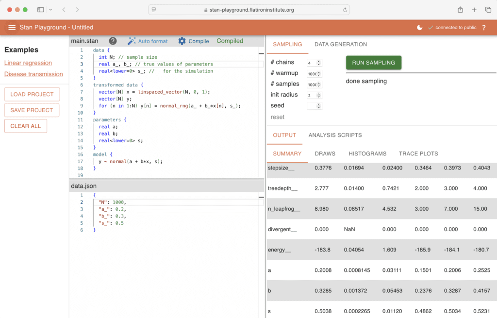
I wrote a simple example that simulates fake data from a linear regression with known parameters (in the transformed data block) and then expresses the log posterior density (in the model block):

data {  int N;             // sample size  real a_, b_;   // true values of parameters  real s_;  //   for the simulation}transformed data {  vector[N] x = linspaced_vector(N, 0, 1);  vector[N] y;  for (n in 1:N) y[n] = normal_rng(a_ + b_*x[n], s_);}parameters {  real a;  real b;  real s;}model {  y ~ normal(a + b*x, s);}

With data:

{  "N": 1000,  "a_": 0.2,  "b_": 0.3,  "s_": 0.5}

It’s so easy

Setting this up a and running it in Stan Playground is the simplest thing in the world:

1. Put the Stan program in the Stan program window. 2. Enter the data (in this case, the sample size of the regression and true parameter values) as a .json in the data window and click to save. 3. In the command window, click once to compile and click again to run. 4. The output (in tabular and graphical form) appears in the output window.

That’s it! The image at the top of this post shows the results.

Also, it catches many bugs in the compilation and sampling stages.