Some thoughts on empirical distributions of z-scores

The z-score is an estimated effect divided by its standard error. The standard error is the estimated standard deviation of the sampling distribution of the estimate. In a clean setting–if the estimate comes from a study with a large sample size, with data that don’t include extreme values, and with an estimate that is linear or asymptotically linear, and the sampling process is correctly modeled–the sampling distribution of the estimate will be approximately normal, and the standard error will be essentially equal to the sampling standard deviation. That is, the sampling distribution of the z-score will be approximately normally distributed with standard deviation of 1. Furthermore, if the estimate is unbiased, then the mean of the sampling distribution of the z-score will be the signal-to-noise ratio, that is, the true effect size divided by the standard error.

Just about all studies are biased in some way, and the way we usually handle this is to retroactively define the true effect size as something like the mean of the sampling distribution of the estimate–that is, the true effect size is defined as the thing that the study is estimating. So if you have a study that’s using a bad measure of exposure, its true effect will typically be lower than the true effect for a study that is measuring exposure more accurately. This is important–we care that studies are not always measuring what they’re trying to measure–but it’s not the focus of our investigation here, which is why we’re taking the “reduced form” approach and considering the target of interest to be the underlying effect size for the studies as they are actually conducted.

The normal approximation to the sampling distribution, and the assumption that the standard error is equal to the standard deviation of the sampling distribution, those too are approximations. I think they are reasonable approximations for the sorts of studies considered here, but we could consider the sensitivity of our findings to relaxing these assumptions in various ways.

So what we’re working with is some published collection of estimates, j=1,…,J, each with a z-score z_j, with the sampling distribution z_j ~ normal(SNR_j, 1), where SNR_j is the signal-to-noise ratio of the true effect from study j. There can be multiple estimates in the published collection from each study but we won’t really worry about that.

Under this model, the distribution of z_j’s across the J estimates–that is, not the sampling distribution for any particular estimate, but the distribution of the collection of J estimates or, equivalently, the distribution of a single z_j drawn at random from this collection of estimates–will look like a convolution of the unit normal distribution and the distribution of the SNR’s.

Mathematically, the convolution of the unit normal distribution with another distribution can look like all sorts of things, but it can’t look like this:

When a large collection of z-scores does look like this–as from the estimates collected by Barnett and Wren (2019), that tells us that one of the above assumptions is wrong.

In this case, the key assumption that is violated was not written above at all! It was the implicit assumption that, first there is some collection of J true effects, thus J signal-to-noise ratios SNR_j, and then for each a z-score is observed, and then all these z-scores are published. The violated assumption is that last part, that all these z-scores are published. The model described above doesn’t account for selection, and obviously there is selection: lots of z-scores between -2 and 2 are missing. To construct the dataset discussed here, Barnett and Wren collected confidence intervals published in papers published in Medline since 1976: “over 968 000 confidence intervals extracted from abstracts and over 350 000 intervals extracted from the full-text.” They write:

The huge excesses of published confidence intervals that are just below the statistically significant threshold are not statistically plausible. Large improvements in research practice are needed to provide more results that better reflect the truth.

And I think that’s right.

The answer to the question, “Why should we care about the distribution of the z-scores of published results?”, is that they tell about two things:

1. The distribution of signal-to-noise ratios for the underlying effects in these studies;

2. The selection process that determines which estimates get reported.

Item #1 is important for two reasons, first because we might be interested in the distribution of true SNRs in some population of studies, and second because we can use an estimated distribution of true SNRs as a prior for Bayesian inference, as Erik and I discuss in our paper from 2022.

Item #2 is also important for two reasons, first because it’s good to understand the processes of scientific reporting and publication–the reported and published results are usually the only ones we hear about–, and second because understand this selection process helps us to adjust for it, especially to account for type M errors or overestimates, an issue that has arisen in psychology, criminology, and many other areas and is directly relevant for policy analysis.

But why talk about the selection effect? Isn’t it obvious?

When you first see the graph of published z-scores, with that big chunk missing between -2 and 2, you might think, sure, that’s what we’d expect, given how the publication game goes. (Some people still argue that it’s fine not to publish non-statistically-significant results because they are uninteresting. I’d prefer to publish everything; but that’s another story. For here, let’s just say that, to the extent there is selection in what is reported and published, we should be accounting for such selection so as to avoid large avoidable errors in our summaries.)

But you don’t always see the pattern with missing values between -2 and 2! Here’s an example:

In our paper in preparation, Witold, Erik, and I look at corpuses of studies from several different sources. The distributions of the z-scores depend on the corpus. Just for example, from Erik’s recent post, here are two distributions, one from PubMed and the other from the Cochrane database of medical trials:

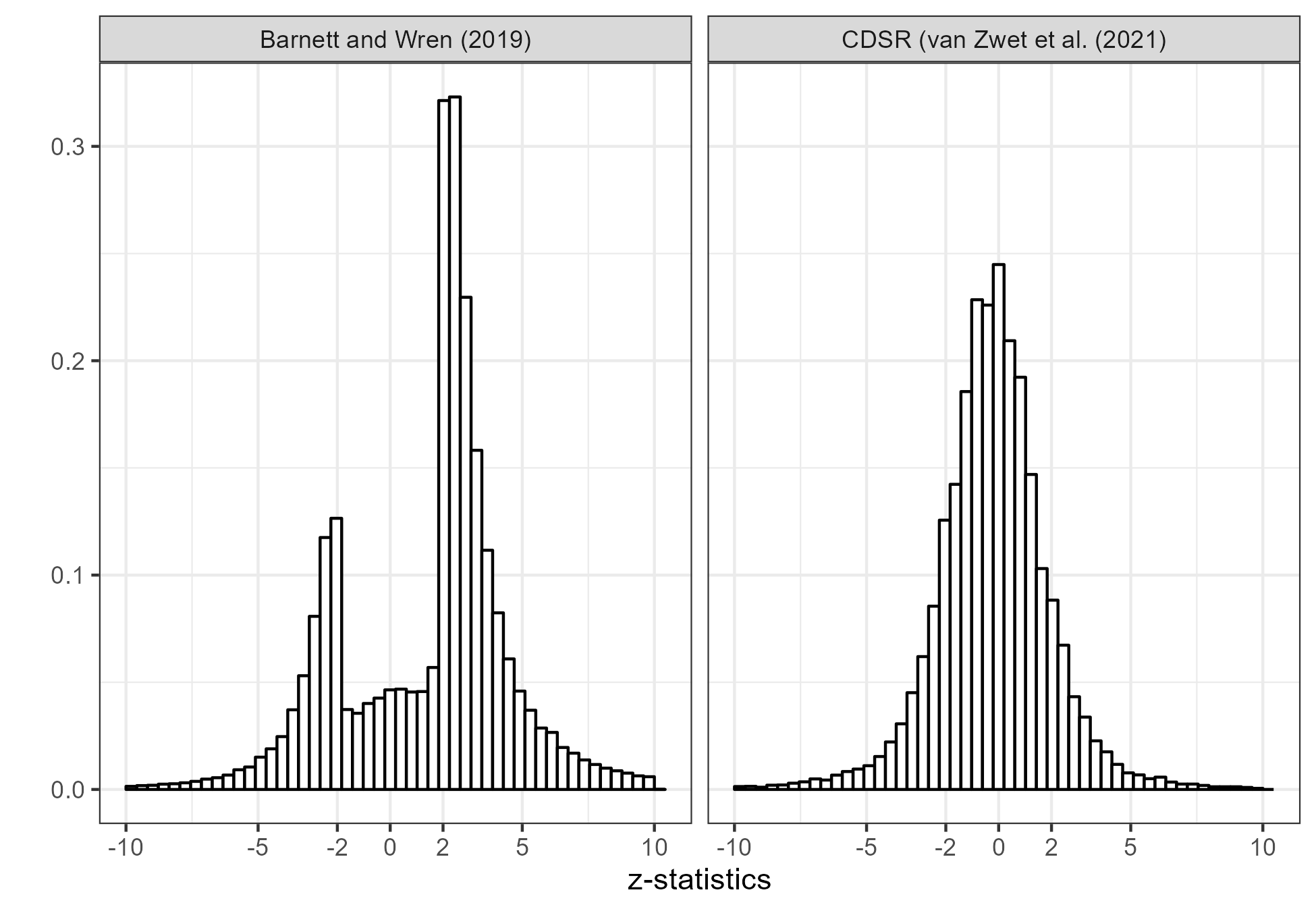
So it’s not automatic that you’ll get that cutout between -2 and 2.

Why look at z-scores rather than p-values?

Our main reason for looking at z-scores rather than p-values is that z has that linear convolution property. Also we think of z as being more generally interpretable, whereas p is interpretable only relative to the null hypothesis. You can think of z as an (unbiased) estimate of SNR with standard error 1.

Wrong intuitions

Applied researchers and statisticians often seem to think that the z-score, or the p-value, is more controllable than it is. With selection, of course, you can control anything, either by waiting until you see the results you want to see, or by sequentially gathering data until you reach some threshold, or by choosing among the many available analyses of your data, or by some combination of these procedures. In the absence of selection, though, you have only a limited amount of control over your z-score. Even if all goes ideally, it will be equal to the true signal-to-noise ratio of your experiment (which you as a researcher do have some control over, although with the limitation that you won’t know the true effect size ahead of time) plus that random unit normal error. So if you’re aiming for a SNR of 2.8 (which will give you 80% power under the usual conditions), your observed z-score could easily be anywhere from 0.8 (corresponding to a p-value of 0.42) and 4.8 (corresponding to a p-value of about 1.6e-6). In real life your SNR will usually be quite a bit less than 2.8, at least so Zwet, Schwab, and Senn estimate based on two corpuses of high-quality studies, which makes sense given that there are lots of reasons that researchers will be over-optimistic regarding effect sizes. (That’s the subject of another post.)

The point is that there’s this intuition that a researcher can, with care, aim for a p-value of about 0.05, or a z-score of about 2. But, no, even if researchers could pinpoint the SNR (which almost always they can’t), the z-score distribution would be blurred.

In theory, you could have a legitimately bimodal distribution of unselected z-scores if true studies were a mix of a distribution of SNRs close to 0 and a distribution of SNRs of 2 or higher, but there’s no evidence whatsoever that this is happening, and lots of evidence that even in high-quality studies, the distribution of SNRs has a peak around zero and gradually declines from there.

Normal sampling distribution != normal distribution of z-scores

In the absence of selection, the distribution of z-scores is approximately the distribution of SNRs convoluted with the unit normal distribution. (One of Erik’s big steps in all this research has been to frame the problem in terms of SNRs rather than effect sizes, which has two benefits: (1) everything is scale-free which allows us to easily set up default procedures, and (2) the math is simpler because we’re convoluting with a fixed normal(0,1) distribution rather than with a different distribution for each estimate.)

This causes some confusion, because there are three distributions: (a) the population distribution of z-scores, which are observed, (b) the population distribution of SNRs, which are unobserved, we can only perform inference for them, and (c) the sampling distribution of each z_j – SNR_j, which is approximately known. Distribution (c) is normal, but there’s no reason to think that (a) or (b) will be normal. Indeed, you can look at the data and there’s direct evidence that distribution (a) has wider tails than normal, which in turn implies wider-than-normal tails for (b). In theory, the distribution of (b) could be anything, but in practice, as noted above, it seems to be unimodal with a peak around zero. Which makes sense, given that any collection of studies is a mixture of all sorts of different things, including some experiments that are very precise and some that are very noisy, and some underlying effect sizes that are large and many that are small.

I think people sometimes get confused between population distributions and sampling distributions. At least, this confusion arises all the time whenever we teach statistics. So when we show a graph of z-scores and then we talk about the z-score having a sampling distribution that’s normal with sd of 1, it’s natural for someone to read this quickly and come out with the impression that we’re saying that the population of z-scores is normal, or that it should be normal. But we’re not.

Thinking continuously rather than discretely

A common theme in our research in this area is to think in terms of continuous effects rather than discretely in terms of effects being zero or nonzero.

We say this for four reasons. Actually, I think more than four, but these are what come to mind right now:

First, in the research areas that interest us, there are lots of effects that are close to zero, but I don’t see sharp divisions between effects that are very close to zero, and effects that are typically small but could be large for some people, and effects that are typically small but could be large in the context of one particular experiment, and effects that are moderate or large across the board, nor can these different scenarios can be reliably distinguished based on experiments designed to estimate an average effect. You’d need huge sample sizes to distinguish zero effects from realistically-sized small but real effects.

Second, studies in the human and environmental sciences typically have some leakage, or bias, or whatever you want to call it. With a big enough sample size, you can find an effect, even if it’s not the effect you’re looking for.

Third, moderate or large effects–or small effects studied carefully–will typically vary among people, across scenarios, and over time, so it’s a mistake to think of nonzero or non-effectively-zero effects as some sort of monolith.

Fourth, we’re looking at signal-to-noise ratios, and these will vary a lot because of variation across studies in measurement quality, resources, and the guessed effect sizes or thresholds used in the study design.

Why I wrote this post

As noted above, Erik, Witold, and I are writing some articles on this and related topics. So maybe it would’ve been better for me to have spent the past two hours working on those articles rather than writing the above post. The reason I wrote and am posting this is: first, sometimes it’s easier to get ideas out in an informal way; second, this way we can communicate with people right now and not have to wait until the article is done; and, third, this is an opportunity for feedback.

So if there’s something confusing about the above post, or if there’s something in it you disagree with, or if you think we missed or dodged any important points, please let us know. Thanks in advance. We’re doing this research for you–it’s our idea of a public service!–so whatever comments you can supply would be helpful. It’s always a challenge to write about points of confusion, because the challenges that make the topic confusing can also make it hard to clarify the problem.

Also, I’ll correct myself when I’ve made mistakes–so, again, if there’s something above that bothers you, let us know, as I’m very open to the possibility that we’re missing something here.

Why does this matter?

The graph at the top of this post is not a scandal in itself. It is what it is. Thousands of people published papers, now collected in Medline, that included confidence intervals. Nothing wrong with looking at these.

The challenge comes in the interpretation. The graph shows a lot of selection: lots of estimates that were less than 2 standard errors from zero were not reported, or were not reported with confidence intervals. It’s important to account for that selection when interpreting published results, whether individually or in aggregate. Accounting for selection is necessary for Bayesian inference (as it is part of the likelihood, the probability of the observed data given the model) and for frequentist inference (as it affects the reference set of problems for which a method will be applied). So, yeah, it’s important. As noted above, I’d prefer to publish everything (and the histogram above from the Cochrane database shows that it is possible to have publication without massive selection on statistical significance), but however things are being published, it’s important to understand the publication and reporting process.

Also, for reasons discussed in the above post we think it makes sense to model the distributions of underlying effects and underlying SNRs as continuous rather than binary.