Survey Statistics: is a mismeasured X better than none at all ?

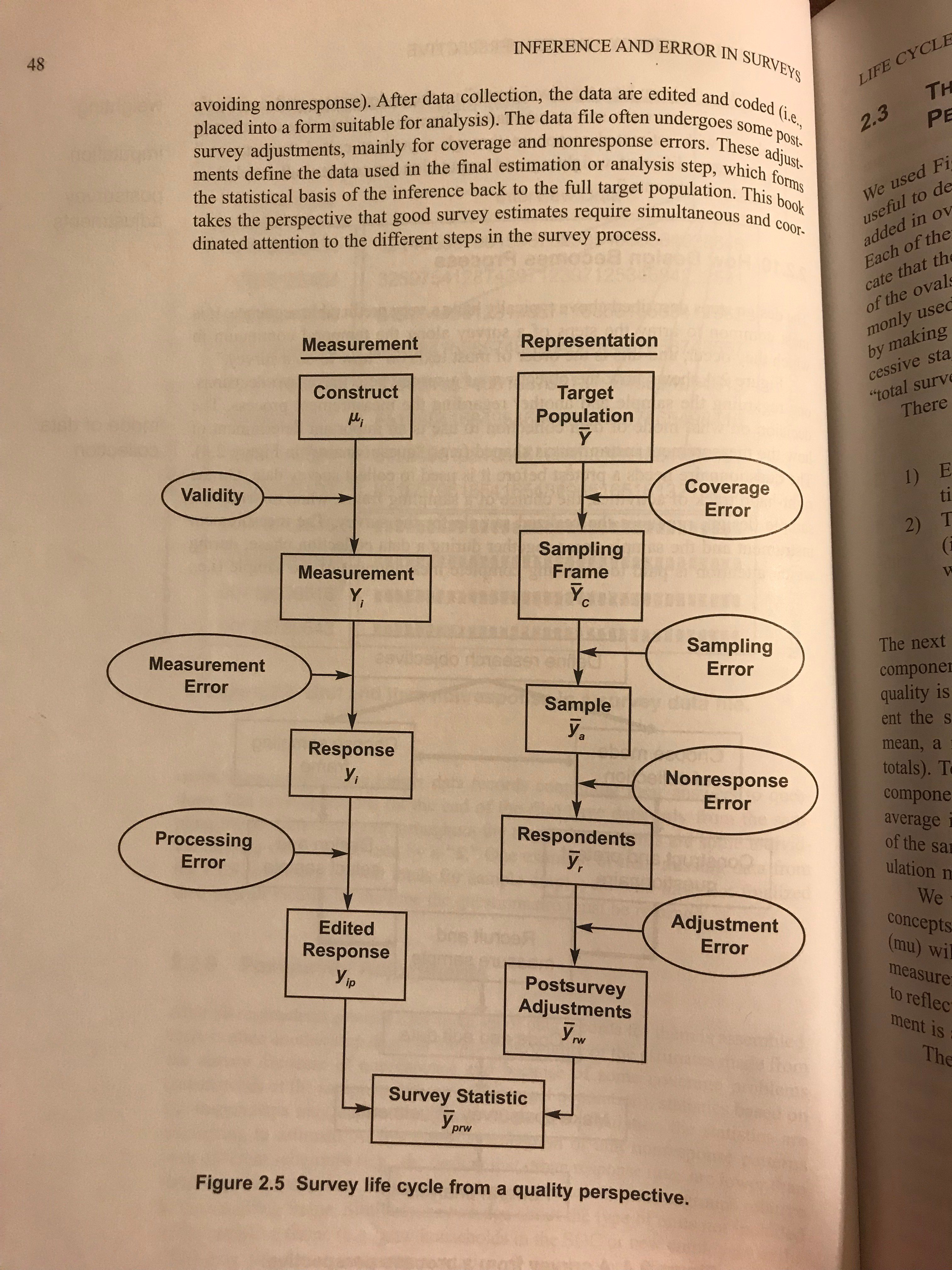
We’ve talked a lot about the “Representation” side of the Groves et al. figure below (also in last month’s holiday-timed blog). Especially nonresponse error.

The “Measurement” side focuses on the gaps between a construct we want to measure (e.g. someone’s current vote choice) and the response we record for them. This concerns what we’ve been calling the “Y” variable.

But there can be measurement problems also with what we’ve been calling the “X” auxiliary variables. Remember poststratification (e.g. MRP), where we attempt to reduce nonresponse bias (on the “Representation” side). We calibrate our estimates of means E[Y] to population data about another variable X, using E[Ehat[Y | X, sample]]. Both X and Y can be mismeasured. Let’s focus today on mismeasured X. Can it still help us ?

Let Y be someone’s current vote choice. It is controversial to adjust for a recalled past vote X* because it might be quite different from actual past vote X. We have population data on X (not X*) from past elections. Why might X and X* differ ? For example, a Harris 2024 voter might say they voted for Trump in 2024 (“winner’s bias”). Or a current (2025) Democrat supporter might say they voted for Harris in 2024, even if they voted for Trump in 2024 (“consistency bias”).

So how might this affect poststratification ? Let’s consider a simple example with only one “X”.

• Y = current 2025 support
• X = true 2024 vote choice
• X* = response for 2024 vote choice

All are binary, = 1 for Democrats and 0 for Republicans.

If by some miracle this one X is enough to handle nonresponse bias, then E[Y | X, sample] = E[Y | X]. So we get the E[Y] we want by E[E[Y | X, sample]]. Let’s write it in an expanded way:

P[X=1] E[Y | X = 1, sample] + P[X = 0] E[Y | X = 0, sample]

We have P[X=1] and P[X=0] from the 2024 election results. But we can’t directly estimate E[Y | X = 1, sample] because we only have X* in the sample.

Consider two choices:

1. Use the imperfect X*: P[X=1] E[Y | X* = 1, sample] + P[X = 0] E[Y | X* = 0, sample]
2. Don’t use it: E[Y | sample]

How would these compare to each other and to the true E[Y] ?

Suppose there is winner’s bias, so some folks voted Democrat (X = 1) but say they didn’t (X* = 0). Folks that still say they voted for Democrats are probably still supportive, so E[Y | X* = 1, sample] might be higher than E[Y | X = 1, sample].

In general, it helps to consider all 4 possible types of folks based on their true X and reported X*. What is the population distribution P[X,X*] ? The distribution in the sample P[X,X* | sample] ? Their Y distribution P[Y = 1 | X,X*] ?

Considering these simple cases helps understand how adjusting for an imperfectly measured past vote could affect results.