When in doubt (in teaching and in research) do a simulation on the computer.

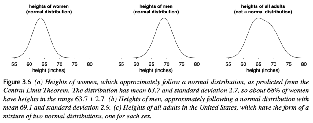
The other day I taught my class and it didn’t go so well. Some students had a question about the central limit theorem–the point is that a sum of many small independent terms will be approximately normally distributed, but that won’t be the case if some of the terms have very long tails or if they have strong dependence or if there is one very large contributor to the sum. I gave as an example the distribution of heights: the distribution of heights of adult women or adult men is approximately normally distributed, but the distribution of heights of all adults is not. This is shown in the above figure from page 41 of Regression and Other Stories.

But this wasn’t so clear to the students. Or, to put it another way: Some students in the class already understood the central limit theorem, and my talking through it in this way didn’t add anything to their understanding; other students in the class had only a vague conception of central limit theorem, and my explanation didn’t help.

This is a not unfamiliar experience for a teacher: you feel like you are talking into a void but it’s not clear what to do next. Keep talking, or just give up.

OK, let me not overstate the problem. The class was not a disaster! This whole episode took only a few minutes, and we moved on. Still, I hate to waste the student’s time, and also I really don’t like to get into this mindless-lecturing vibe. I was just parroting the explanation of the central limit theorem that was already in print, and it would’ve been better for me to have just pointed the students to the relevant page in the book and then move on.

But there’s another way–as I remembered on the walk back to my office after the class was over.

It’s always an option to do a simulation on the computer. It’s win-win: you’re teaching programming as well as statistics, and also the code you write provides an opening for students to explore further on their own.

Here’s an example. First I set things up to perform a simulation and display multiple graphs:

par(mfrow=c(2,2), mar=c(3,3,1,1), mgp=c(1.5,.5,0))set.seed(123)

Then I simulate a million instances of a random variable formed by adding 10 little pieces:

N <- 1e6K <- 10y_individual <- array(NA, c(N,K))for (k in 1:K){  y_individual[,k] <- runif(N, 0, 1)}y_sum <- rowSums(y_individual)

This should look a lot like a normal distribution:

hist(y_sum)

I then add a big fat new term so it won't look normal anymore:

y_sum_2 <- y_sum + 10*rbinom(N, 1, 0.5)hist(y_sum_2)

These are almost too separated to be convincing so I try a smaller separation:

y_sum_2 <- y_sum + 3*rbinom(N, 1, 0.5)hist(y_sum_2)

To get something more interesting I can move them together and give the two modes unequal weight:

y_sum_2 <- y_sum + 2*rbinom(N, 1, 0.4)hist(y_sum_2)

Lots more could be done. The point is that I could do the above in a few minutes and it provides the basis for student input. For example, I could ask students to work in pairs and try to come up with other ways to defeat the central limit theorem. This will be much clear with runnable code than with me scrawling math on the blackboard.

I've already said that how much I like simulated-data experimentation when doing applied or methodological research . . . ummm, here are some old posts on the topic:

- Fake-data simulation as posterior predictive checking: A formalization of the folk theorem of statistical computing!

- Why I like hypothesis testing (it’s another way to say “fake-data simulation”):

- (What’s So Funny ‘Bout) Fake Data Simulation

- Simulated-data experimentation: Why does it work so well?

- Yes, I really really really like fake-data simulation, and I can’t stop talking about it.

And that last post has a bunch more old links at the end.