Survey Statistics: 4th helpings of the logit shift

In June 2025 we discussed 2 flavors of calibration, including “the logit shift”. In August 2025 we took 2nd helpings of the logit shift, focusing on multinomial outcomes. In December 2025 we took 3rd helpings, focusing on multivariate outcomes. Maybe folks have had enough (I was the only person to comment on the 3rd helpings post). But G. Elliott Morris linked to the new Will Marble and Josh Clinton multivariate logit-shifting paper, which reminded me to think about it again.

They consider the 2022 midterms in Michigan:

• y_1 = governor vote choice
• y_2 = abortion proposition vote choice
• x = demographics

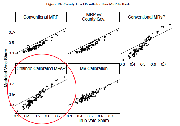
They estimate E(y_2 | county) and compare it to known truth. They have y_1, y_2, x in a survey, x in the population, and E(y_1 | county). Will and Josh look at a few estimation methods, including “Chained Calibrated MrsP“:

• Add y_1 to the population data: fit p(y_1 | x) from the survey, logit-shift to E(y_1 | county).
• MRP: fit p(y_2 | y_1, x) from the survey, average over the population distribution of y_1, x

Kuriwaki et al. 2024 do this, as we discussed in June 2025. Our mystery from December 2025 was why this method seems to do poorly in Will and Josh‘s paper:

Will suspected it was due to Jensen’s inequality, so I wrote a silly simulation to try to understand that.

n_county <- 50n_per <- 500b <- 8a_county <- rnorm(n_county, -3, 2.5)p <- runif(n_county, 0.3, 0.7)county <- rep(1:n_county, each = n_per)y1 <- rbinom(n_county * n_per, 1, p[county])true_E <- tapply(seq_along(y1), county, function(ix)mean(plogis(a_county[county[ix[1]]] +b*y1[ix])))jensen_ignored <- plogis(a_county + b * tapply(y1, county, mean))plot(true_E, jensen_ignored,     xlab="True E[logit^-1(a + b*y1) | county]",     ylab="logit^-1(a + b*E[y1|county])",     pch=16,xlim=c(0,1),ylim=c(0,1))abline(0, 1, col = "red", lwd = 2)

Thoughts ? Have you had enough of the logit-shift ?