Bowie integrator and the nonlinear pendulum
The Endeavour 2025-12-23
I recently learned of Bowie’s numerical method for solving ordinary differential equations of the form
y″ = f(y)
via Alex Scarazzini’s masters thesis [1].
The only reference I’ve been able to find for the method, other than [1], is the NASA Orbital Flight Handbook from 1963. The handbook describes the method as “a method employed by C. Bowie and incorporated in many Martin programs” and says nothing more about its origin.
Martin Company
What does it mean by “Martin programs”? The first line of the foreword of the manual says
This handbook has been produced by the Space Systems Division of the Martin Company under Contract NAS8-S03l with the George C. Marshall Space Flight Center of the National Aeronautics and Space Administration.
The Martin Company was the Glenn L. Martin Company, which became Martin Marietta after merging with American-Marietta Corporation in 1961. The handbook was written after the merger but used the older name. Martin Marietta would go on to become Lockheed Martin in 1995.
Bowie’s method was used “in many Martin programs” and yet is practically unknown in academic circles. Scarazzini’s thesis shows the method works well for his problem.
Nonlinear pendulum
My first thought when I saw the form of differential equations Bowie’s method solves was the nonlinear pendulum equation
y″ = − sin(y)
where the initial displacement y(0) is too large for the approximation sin θ ≈ θ to be sufficiently accurate. I wrote some Python code to try out Bowie’s method on this equation.
import numpy as npN = 100y = np.zeros(N)yp = np.zeros(N) # y'y[0] = 1yp[0] = 0T = 4*ellipk(np.sin(y[0]/2)**2)h = T/Nf = lambda x: -np.sin(x)fp = lambda x: -np.cos(x) # f'fpp = lambda x: np.sin(x) # f''for n in range(0, N-1): y[n+1] = y[n] + h*yp[n] + 0.5*h**2*f(y[n]) + \ (h**3/6)*fp(y[n])*yp[n] + \ (h**4/24)*(fpp(yp[n])**2 + fp(y[n])*f(y[n])) yp[n+1] = yp[n] + h*f(y[n]) + 0.5*h**2*fp(y[n])*yp[n] + \ (h**3/6)*(fpp(yp[n])**2 + fp(y[n])*f(y[n]))
Here’s a graph of the numerical solution.
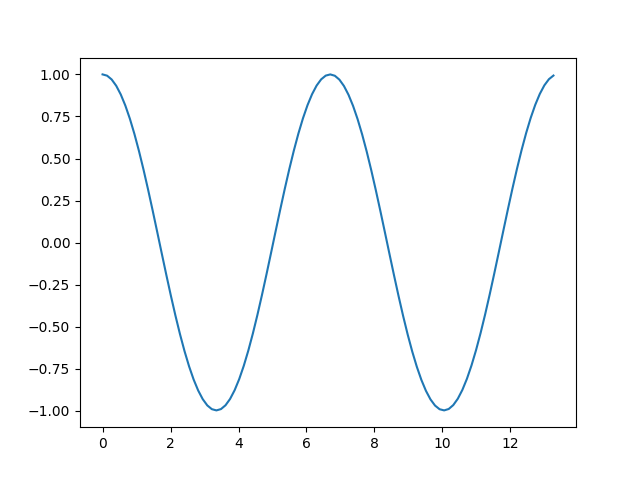
The solution looks like a cosine, but it isn’t exactly. As I explain here,
The solution to the nonlinear pendulum equation is also periodic, though the solution is a combination of Jacobi functions rather than a combination of trig functions. The difference between the two solutions is small when θ0 is small, but becomes more significant as θ0 increases.
The difference in the periods is more evident than the difference in shape for the two waves. The period of the nonlinear solution is longer than that of the linearized solution.
That’s why the period T in the code is not
2π = 6.28
but rather
4 K(sin² θ0/2) = 6.70.
You’ll also see the period of the nonlinear pendulum given as 4 K(sin θ0/2). As pointed out in the article linked above,
There are two conventions for defining the complete elliptic integral of the first kind. SciPy uses a convention for K that requires us to square the argument.
Related posts
[1] Alex Scarazzini.3D Visualization of a Schwarzschild Black Hole Environment. University of Bern. August 2025.
The post Bowie integrator and the nonlinear pendulum first appeared on John D. Cook.