Estimating Reliability – Psychometrics
R-bloggers 2013-04-03
(This article was first published on Econometrics by Simulation, and kindly contributed to R-bloggers)
 # Each item has a item characteristic curve (ICC) of: PL3 = function(theta,a, b, c) c+(1-c)*exp(a*(theta-b))/(1+exp(a*(theta-b))) # Let's imagine we have a test with parameters a,b,c nitems = 50 test.a = rnorm(nitems)*.2+1 test.b = rnorm(nitems) test.c = runif(nitems)*.3 # I classical test theory we have the assumption that total variance of the test results is equal to the variance of the true scores (defined as the expected outcome of the test for a given subject) plus measurement error [Var(X) = Var(T(theta)) + Var(E)]. # We "know" that classical test theory is wrong because we know that the error must be a function of ability (theta) since we know that no matter how good (or bad) a student is, the student will never get above the maximum (or below the minimum) score of the test. # Let's generate the student pool. nstud = 5000 stud.theta = rnorm(nstud) # First let's generate our expected outcomes by student. prob.correct = matrix(NA, ncol=nitems, nrow=nstud) for (i in 1:nitems) prob.correct[,i]=PL3(stud.theta, test.a[i], test.b[i], test.c[i]) # Generate true scores true.score = apply(prob.correct, 1, sum) # Generate a single sample item responses for test 1. x1.responses = matrix(runif(nitems*nstud), ncol=nitems, nrow=nstud) # Generate total scores x1.score = apply(x1.responses, 1, sum) # The test sampling seems to be working correctly cor(true.score, x1.score) # Let's sample a parrellel test x2.responses = matrix(runif(nitems*nstud), ncol=nitems, nrow=nstud) # Generate total scores x2.score = apply(x2.responses, 1, sum) # Classical reliability is defined as the correlation between two parrellel test scores (I think): rel.XX = cor(x1.score, x2.score) # Looks like our estimated reliability is about .84 or .85 plot(x1.score, x2.score, main="Highly Reliable Test fit along a 45 degree line")
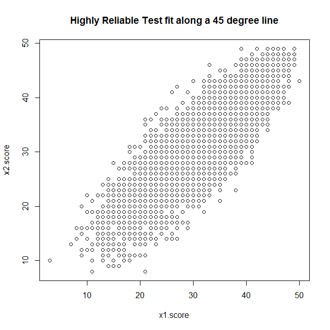
To leave a comment for the author, please follow the link and comment on his blog: Econometrics by Simulation.
R-bloggers.com offers daily e-mail updates about R news and tutorials on topics such as: visualization (ggplot2, Boxplots, maps, animation), programming (RStudio, Sweave, LaTeX, SQL, Eclipse, git, hadoop, Web Scraping) statistics (regression, PCA, time series,ecdf, trading) and more...