Adding Percentiles to PDQ

PQD performs a mean value analysis of queueing network models: mean values in; mean values out. By mean, I mean statistical mean or average. Mean input values include such queueing metrics as service times and arrival rates. These could be sample means. Mean output values include such queueing metrics as waiting time and queue length. These are computed means based on a known distribution. I'll talk about what distribution, shortly. Sometimes you might also want to report measures of dispersion about those mean values, e.g., the 90th or 95th percentiles.

Percentile Rules of Thumb

In The Practical Performance Analyst (1998, 2000) and Analyzing Computer System Performance with Perl::PDQ (2011), I offer the following Guerrilla rules of thumb for percentiles, based on a mean residence time R:

• 80th percentile: p80 ≃ 5R/3
• 90th percentile: p90 ≃ 7R/3
• 95th percentile: p95 ≃ 9R/3

I could also add the 50th percentile or median: p50 ≃ 2R/3, which I hadn't thought of until I was putting this blog post together.

Example: Cellphone TTFF

As an example of how the above rules of thumb might be applied, an article in GPS World discusses how to calculate the time-to-first-fix or TTFF for cellphones.

It can be shown that the distribution of the acquisition time of a satellite, at a given starting time, can be approximated by an exponential distribution. This distribution explains the non-linearity of the relationship between the TTFF and the probability of fix. In our example, the 50-percent probability of fix was about 1.2 seconds. Moving the requirement to 90 percent made it about 2 seconds, and 95 percent about 2.5 seconds.

In other words:

• 50th percentile: p50 = 1.2 seconds
• 90th percentile: p90 = 2.0 seconds
• 95th percentile: p95 = 2.5 seconds

I can assess these values Guerrilla-style by applying the above rules of thumb in R:

 pTTFF  return(c(2*R/3, 5*R/3, 7*R/3, 9*R/3)) } # Choose R = 0.83333 (maybe from 1/1.2 ???) > pTTFF(0.8333) [1] 0.5555333 1.3888333 1.9443667 2.4999000 

Something is out of whack! The p90 and p95 values agree, well enough, but p50 does not. It could be a misprint in the article, maybe my choice of R is wrong, etc. Whatever the source of the discrepancy, it has to be explained. That's why being able to go Guerrilla is important. Even having wrong expectations is better than having no expectations.

Quantiles in R

The Guerrilla rules of thumb follow from the assumption that the underlying statistics are exponentially distributed. The exponential PDF and corresponding exponential CDF are shown in Fig. 1, where the mean value, R = 1 (red line), is chosen for convenience.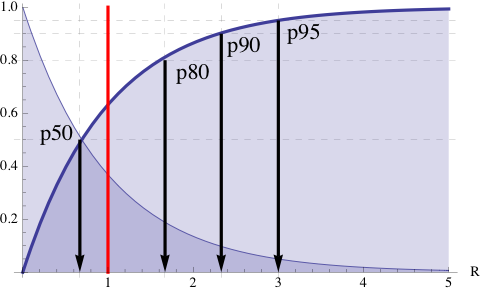

Figure 1. PDF and CDF of the exponential distribution

The CDF gives the probabiites and therefore is bounded between 0 and 1 on the y-axis so that the corresponding percentiles can be read off directly from the appropriate horizontal dashed line and its corresponding vertical arrow. The exact values can be determined using the qexp function in R.

 > qexp(c(0.50, 0.80, 0.90, 0.95)) [1] 0.6931472 1.6094379 2.3025851 2.9957323 

which can be compared with the locations on the x-axis in Fig. 1 where the arrowheads are pointing.

Example: PDQ with Exact Percentiles

The rules of thumb and the exponential assumption are certainly valid for M/M/1 queues in any PDQ model. However, rather than clutter up the standard PDQ Report with all these percentiles, it is preferable to select the PDQ output metrics of interest and add their corresponding percentiles in a custom format. For example:

 library(pdq) arrivalRate serviceTime Init("M/M/1 queue")                # initialize PDQ CreateOpen("Calls", arrivalRate)   # open network CreateNode("Switch", CEN, FCFS)    # single server in FIFO order SetDemand("Switch", "Calls", serviceTime) Solve(CANON)                       # Solve the model #Report() pdqR cat(sprintf("Mean R: %2.4f seconds\n", pdqR)) cat(sprintf("p50  R: %2.4f seconds\n", qexp(p=0.50,rate=1/pdqR))) cat(sprintf("p80  R: %2.4f seconds\n", qexp(p=0.80,rate=1/pdqR))) cat(sprintf("p90  R: %2.4f seconds\n", qexp(p=0.90,rate=1/pdqR))) cat(sprintf("p95  R: %2.4f seconds\n", qexp(p=0.95,rate=1/pdqR))) 

which computes the following PDQ outputs:

 Mean R: 0.8333 seconds p50  R: 0.5776 seconds p80  R: 1.3412 seconds p90  R: 1.9188 seconds p95  R: 2.4964 seconds 

The same approach can be extended to multi-server queues defined through the PDQ function CreateMultiNode(), but qexp has to be replaced with: \begin{equation*} p_{m}(q) = \dfrac{R}{m(1-\rho)} \log \bigg[ \dfrac{C(m,m\rho)}{1-q} \bigg] \end{equation*} where $C$ is the Erlang C-function, $\rho$ is the per-server utilization and $q$ is the desired quantile. If enough interest is expressed, I can add such a function to a future release of PDQ. I'll say more in the upcoming Guerrilla data analysis class.