Railway population

R-bloggers 2026-01-04

[This article was first published on r.iresmi.net, and kindly contributed to R-bloggers]. (You can report issue about the content on this page here)

Want to share your content on R-bloggers? click here if you have a blog, or here if you don't.

Eurostar 3213 and 3214 in Marseille-Saint-Charles in 2017 – CC-BY by Roel Hemkes

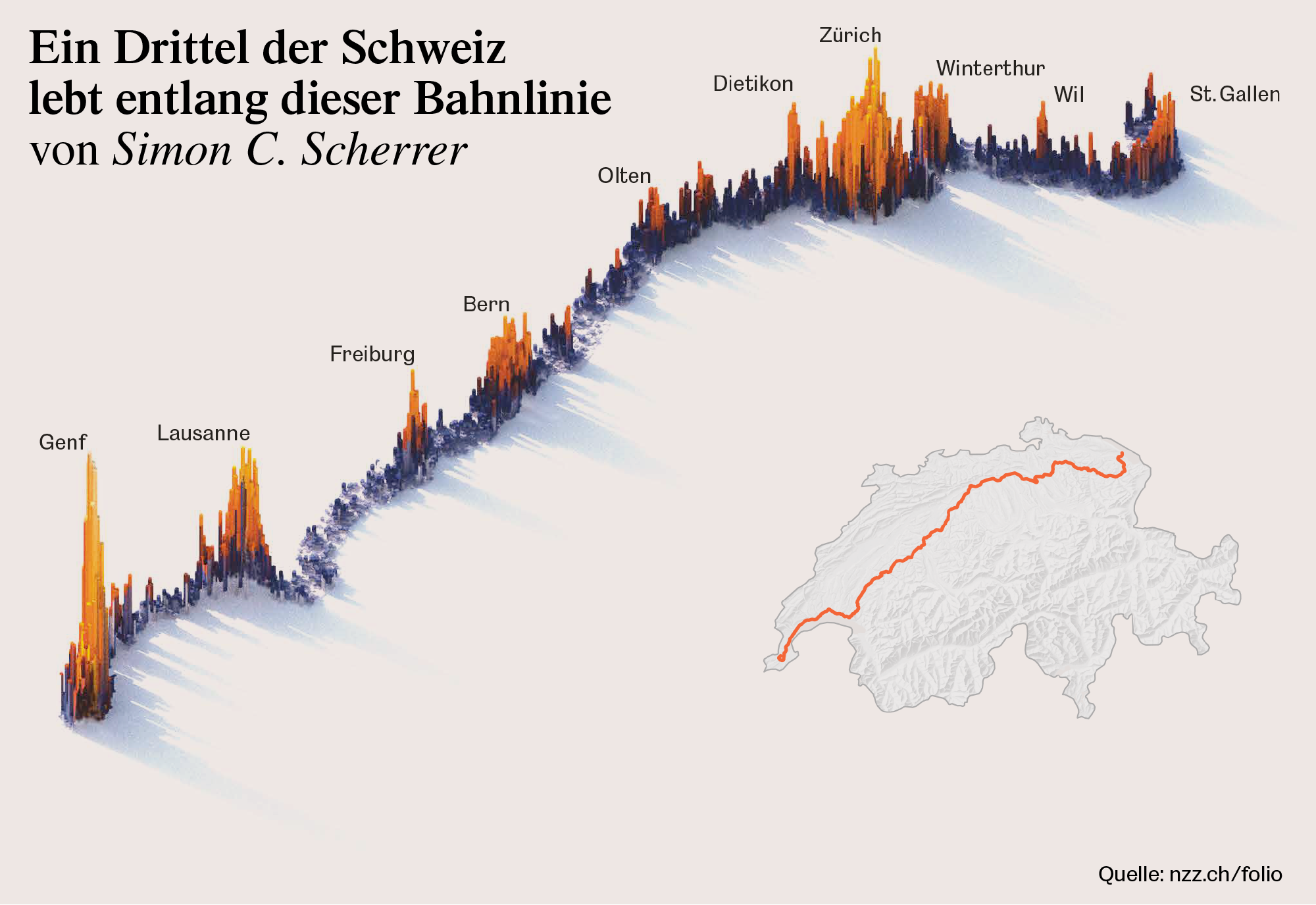
The following map from 2024 by Simon C. Scherrer (via @freakonometrics) indicates that one-third of the Swiss population lives in a five-kilometer-wide strip on either side of the Intercity 1 railway line.

A third of the Switzerland population lives along the Geneva–St. Gallen railway line – 2024-04-24 by Simon C. Scherrer – data: Kontur/data.sbb.ch/Natural Earth

What is the situation in France?

I didn’t easily find the statistics per line, but I guess a similar configuration —main line (whatever it means), main cities, many passengers, crossing the country— would be the discontinued Eurostar (London)–Calais–Lille–Marne-la-Vallée–Lyon–Marseille or the current TGV inOui Lille-Lyon-Marseille. However they don’t stop at Paris intra muros, so we miss a good part of the population.

Config

library(sf)library(glue)library(dplyr)library(osmdata)library(purrr)library(httr2)library(rnaturalearth)library(stringr)library(ggplot2)sf_use_s2(FALSE)

Note

A 7z system binary is also required

Data

Railway

We can get the railway geometry from the OSM relation with {osmdata} and an Overpass API query.

osm <- r"([out:xml][timeout:6000];relation(5951791);(._;>;);out body;)" |>   osmdata_sf() eurostar <- osm |>   pluck("osm_multilines")stations <- osm$osm_points |>   filter(railway == "stop",          uic_ref %in% c("8775100", "8772319", "8711184", "8722326"))

fr <- ne_countries(scale = "large") |>   st_intersection(eurostar |>                     st_bbox() |>                     st_as_sfc() |>                     st_buffer(4.5, joinStyle = "MITRE", mitreLimit = 10))eurostar |>   ggplot() +  geom_sf(data = fr, color = "darkgrey") +  geom_sf(color = "red", linewidth = 0.5, alpha = 0.8) +  geom_sf(data = stations) +  geom_sf_text(data = stations,                aes(label = str_wrap(name, width = 15,                                    whitespace_only = FALSE)),                size = 3,               hjust = 1.1) +  labs(title = "London-Marseille",       caption = glue("data: OpenStreetMap contributors                      Natural Earth                      https://r.iresmi.net - {Sys.Date()}")) +  theme_void() +  theme(plot.caption = element_text(size = 7, color = "grey40"),        plot.background = element_rect(fill = "white"),        plot.margin = unit(c(.2, .2, .2, .2), units = "cm"))

Figure 1: London-Marseille railway

Population

Population comes from INSEE 2015 200 m grid.

Caution

The 7z file is itself zipped!

if (!file.exists("carreaux_200m_met.gpkg")) {  pop_file <- "Filosofi2019_carreaux_200m_gpkg.zip"  if (!file.exists(pop_file)) {    request(glue("https://www.insee.fr/fr/statistiques/fichier/7655475/\\                 {pop_file}")) |>       req_perform(pop_file)  }  unzip(pop_file)  system("7z e Filosofi2019_carreaux_200m_gpkg.7z carreaux_200m_met.gpkg")  system("rm Filosofi2019_carreaux_200m_gpkg.*")}pop <- read_sf("carreaux_200m_met.gpkg")

Results

Within 5 km

pop_5km <- pop |>   st_filter(eurostar |>               st_transform("EPSG:2154") |>               st_buffer(5000)) |>   st_drop_geometry() |>   summarise(pop_tot = sum(ind, na.rm = TRUE)) |>   pull(pop_tot)pop_fr <- pop |>   st_drop_geometry() |>   summarise(pop_tot = sum(ind, na.rm = TRUE)) |>   pull(pop_tot)

Total population: 62,971,073
Population within 5 km: 4,163,426

So only 6.6 % of the french (metropolitan) population is within 5 km of this railway line.

Within 50 km

If we extend to 50 km, we’ll capture most part of Paris…

pop_50km <- pop |>   st_filter(eurostar |>               st_transform("EPSG:2154") |>               st_buffer(50000)) |>   st_drop_geometry() |>   summarise(pop_tot = sum(ind, na.rm = TRUE)) |>   pull(pop_tot)

Population within 50 km: 25,696,130

So 40.8 % of the french (metropolitan) population is within 50 km of this railway line. Not bad, but the question could be now: does the train stop at a station near you? This is left as an exercise to the reader (spoiler: less and less…).

eurostar |>   ggplot() +  geom_sf(data = fr, color = "darkgrey") +  geom_sf(color = "red", linewidth = 0.5, alpha = 0.8) +  geom_sf(data = eurostar |>             st_transform("EPSG:2154") |>             st_buffer(50000),          fill = "red", alpha = 0.2) +  geom_sf(data = stations) +  geom_sf_text(data = stations,                aes(label = str_wrap(name, width = 15,                                    whitespace_only = FALSE)),                size = 3,               hjust = 1.1) +  labs(title = "London-Marseille",       caption = glue("data: OpenStreetMap contributors                      Natural Earth                      https://r.iresmi.net - {Sys.Date()}")) +  theme_void() +  theme(plot.caption = element_text(size = 7, color = "grey40"),        plot.background = element_rect(fill = "white"),        plot.margin = unit(c(.2, .2, .2, .2), units = "cm"))

Map of London-Marseille railway and a 50 km buffer

Figure 2: London-Marseille railway in France and a 50 km buffer

To leave a comment for the author, please follow the link and comment on their blog: r.iresmi.net.

R-bloggers.com offers daily e-mail updates about R news and tutorials about learning R and many other topics. Click here if you're looking to post or find an R/data-science job.

Want to share your content on R-bloggers? click here if you have a blog, or here if you don't.

Continue reading: Railway population