Hamilton Regime Switching Model using R code
R-bloggers 2022-02-17
[This article was first published on K & L Fintech Modeling, and kindly contributed to R-bloggers]. (You can report issue about the content on this page here)
Want to share your content on R-bloggers? click here if you have a blog, or here if you don't.
This post estimates parameters of a regime switching model directly by using R code. The same model was already implemented by using MSwM R package in the previous post. Through this hand-on example I hope we can learn the process of Hamilton filtering more deeply. Want to share your content on R-bloggers? click here if you have a blog, or here if you don't.
Hamilton Regime Switching Model using R code
In the previous post below, we used MSwM R package to estimate parameters of the two-state regime switching model. In this post we directly estimate it with the sequence of Hamilton filter.Regime Switching model
A two-state regime switching linear regression model and a transition probability matrix are of the following forms. \[\begin{align} &y_t = c_{s_t} + \beta_{s_t}x_t + \epsilon_{s_t,t}, \quad \epsilon_{s_t,t} \sim N(0,\sigma_{s_t}) \\ \\ &P(s_t=j|s_{t−1}=i) = P_{ij} = \begin{bmatrix} p_{00} & p_{01} \\ p_{10} & p_{11} \end{bmatrix} \end{align}\] Here \(s_t\) can take on 0 or 1 and \(p_{ij}\) is the probability of transitioning from regime \(i\) at time \(t-1\) to regime \(j\) at time \(t\).Hamilton Filtering
Hamilton filter is of the following sequence as we presented it in the previous post. 1) \(t-1\) state (previous state) \[\begin{align} \xi_{i,t-1} &= P(s_{t-1} = i|\tilde{y}_{t-1};\mathbf{\theta}) \end{align}\] 2) state transition from \(i\) to \(j\) (state propagation) \[\begin{align} p_{ij} \end{align}\] 3) densities under the two regimes at \(t\) (data observations and state dependent errors) \[\begin{align} \eta_{jt} = \frac{1}{\sqrt{2\pi}\sigma}\exp\left[-\frac{(y_t-c_j-\beta_j x_t)^2}{2\sigma_j^2}\right] \end{align}\] 4) conditional density of the time \(t\) observation (combined likelihood with state being collapsed): \[\begin{align} f(y_t|\tilde{y}_{t-1};\mathbf{\theta}) &= \xi_{0,t-1}p_{00}\eta_{0t} + \xi_{0,t-1}p_{01}\eta_{1t} \\ &+ \xi_{1,t-1}p_{10}\eta_{0t} + \xi_{1,t-1}p_{11}\eta_{1t} \end{align}\] 5) \(t\) posterior state (corrected from previous state) \[\begin{align} \xi_{jt} = \frac{\sum_{i=0}^{1} \xi_{i,t-1}p_{ij}\eta_{jt}} {f(y_t|\tilde{y}_{t-1};\mathbf{\theta})} \end{align}\] 6) use posterior state at time \(t\) as previous state a time \(t+1\) (substitution) \[\begin{align} \xi_{jt} \rightarrow \xi_{i,t-1} \end{align}\] 7) iterate 1) ~ 6) from t = 1 to T As a result of executing this iteration, the sample conditional log likelihood of the observed data can be calculated in the following way. \[\begin{align} \log f(\tilde{y}_{t}|y_0;\mathbf{\theta}) = \sum_{t=1}^{T}{ f(y_t|\tilde{y}_{t-1};\mathbf{\theta}) } \end{align}\] With this log-likelihood function, we use a numerical optimization to find the best fitting parameter set(\(\tilde{\mathbf{\theta}}\)).Numerical Optimization
To start iterations of the Hamilton filter, we need to set \(\xi_{i,0} \) and in most cases the unconditional state probabilities are used. \[\begin{align} \xi_{0,0} &= \frac{1 – p_{11}}{2 – p_{00} – p_{11}} \\ \xi_{1,0} &= 1 – \xi_{0,0} \end{align}\]R code
The following R code implement MLE parameter estimation of two-state regime switching model with the same date as in the previous post. This code is line with the process of the Hamilton filtering.#========================================================#
# Quantitative ALM, Financial Econometrics & Derivatives
# ML/DL using R, Python, Tensorflow by Sang-Heon Lee
#
# https://kiandlee.blogspot.com
#——————————————————–#
# Hamilton Regime Switching Model – AR(1) inflation model
#========================================================#
graphics.off() # clear all graphs
rm(list = ls()) # remove all files from your workspace
library(MSwM)
#——————————————
# Data : U.S. CPI inflation 12M, yoy
#——————————————
inf <– c(
3.6536,3.4686,2.9388,3.1676,3.5011,3.144,2.6851,2.6851,2.5591,
2.1053,1.8767,1.5909,1.1888,1.13,1.3537,1.6306,1.2332,1.0635,
1.455,1.7324,1.5046,2.0068,2.2285,2.45,2.7201,3.0976,2.9804,
2.1518,1.8764,1.93,2.0347,2.1919,2.3505,2.0214,1.91,2.0148,
2.006,1.6744,1.7251,2.2667,2.8566,3.1185,2.8972,2.5155,2.5075,
3.1411,3.5576,3.2877,2.8052,3.0073,3.1565,3.3065,2.8289,2.5093,
3.0211,3.582,4.6328,4.2581,3.284,3.284,3.9401,3.5736,3.3608,
3.5501,3.9002,4.0967,4.0227,3.8514,1.9921,1.3965,1.9496,2.4927,
2.0545,2.3914,2.7598,2.5599,2.6738,2.6571,2.2914,1.8797,2.7944,
3.547,4.2803,4.0266,4.205,4.0594,3.8979,3.8295,4.007,4.818,
5.3517,5.1719,4.8345,3.6631,1.0939,–0.0222,–0.1137,0.0085,–0.4475,
–0.578,–1.021,–1.2368,–1.9782,–1.495,–1.3875,–0.2242,1.8965,2.7753,
2.5873,2.1285,2.2604,2.1828,1.9837,1.1153,1.3319,1.1436,1.1121,
1.1599,1.0787,1.4276,1.6865,2.1026,2.5855,3.0308,3.4005,3.4424,
3.5173,3.6862,3.7417,3.4617,3.3932,3.0161,2.9644,2.857,2.5501,
2.2477,1.723,1.6403,1.4076,1.6719,1.931,2.1328,1.7801,1.7442,
1.67,1.998,1.5073,1.1324,1.3808,1.7012,1.8679,1.5271,1.0888,
0.873,1.2253,1.5015,1.5458,1.1142,1.5998,1.9951,2.1438,2.0381,
1.955,1.7006,1.67,1.5967,1.224,0.651,–0.2302,–0.0871,–0.022,
–0.1041,0.035,0.1794,0.2254,0.241,0.0088,0.1275,0.4354,0.6367,
1.2299,0.8437,0.8877,1.1658,1.0727,1.0735,0.8646,1.0498,1.5368,
1.6719,1.6703,2.0301,2.4802,2.7167,2.3602,2.186,1.866,1.6498,
1.7255,1.9187,2.2042,2.0132,2.1872,2.0797,2.0722,2.2013,2.3318,
2.427,2.7149,2.7997,2.8511,2.6282,2.2586,2.4991,2.1768,1.902,
1.4846,1.461,1.8386,1.9981,1.8117,1.6863,1.8058,1.7261,1.7098,
1.7591,2.0231,2.2363,2.4441,2.2881,1.5004,0.3386,0.2233,0.7252,
1.0414,1.3161,1.4001,1.1876,1.1324,1.2918,1.3607,1.6618,2.6031,
4.0692,4.809,5.1876,5.1478,5.0717,5.2377,6.0564,6.6541,6.8811)
ninf <– length(inf)
# y and its first lag
y0 <– inf[2:ninf]; y1 <– inf[1:(ninf–1)]
df <– data.frame(y = y0, y1 = y1)
#——————————————
# Single State : OLS
#——————————————
lrm <– lm(y~y1,df)
#——————————————
# Two State : Markov Switching (MSwM)
#——————————————
k <– 2 # two-regime
mv <– 3 # means of 2 variables + 1 for volatility
rsm=msmFit(lrm, k=2, p=0, sw=rep(TRUE, mv),
control=list(parallel=FALSE))
#——————————————
# function : Hamilton filter
#——————————————
# y = const0 + beta0*x + e0,
# y = const1 + beta1*x + e1,
#
# e0 ~ N(0,sigma0) : regime 1
# e1 ~ N(0,sigma1) : regime 2
##——————————————
hamilton.filter <– function(param,x,y){
# param = mle$par; x = y1; y = y0
nobs = length(y)
# constant, AR(1), sigma
const0 <– param[1]; const1 <– param[2]
beta0 <– param[3]; beta1 <– param[4]
sigma0 <– param[5]; sigma1 <– param[6]
# restrictions on range of probability (0~1)
p00 <– 1/(1+exp(–param[7]))
p11 <– 1/(1+exp(–param[8]))
p01 <– 1–p00; p10 <– 1–p11
# previous and updated state (fp)
ps_i0 <– us_j0 <– ps_i1 <– us_j1 <– NULL
# steady state probability
sspr1 <– (1–p00)/(2–p11–p00)
sspr0 <– 1–sspr1
# initial values for states (fp0)
us_j0 <– sspr0
us_j1 <– sspr1
# predicted state, filtered and smoothed probability
ps <– fp <– sp <– matrix(0,nrow = length(y),ncol = 2)
loglike <– 0
for(t in 1:nobs){
#) t-1 state (previous state)
# -> use previous updated state
ps_i0 <– us_j0
ps_i1 <– us_j1
# 2) state transition from i to j (state propagation)
# -> use time invariant transition matrix
# 3) densities under the two regimes at t
# (data observations and state dependent errors)
# regression error
er0 <– y[t] – const0 – beta0*x[t]
er1 <– y[t] – const1 – beta1*x[t]
eta_j0 <– (1/(sqrt(2*pi*sigma0^2)))*exp(–(er0^2)/(2*(sigma0^2)))
eta_j1 <– (1/(sqrt(2*pi*sigma1^2)))*exp(–(er1^2)/(2*(sigma1^2)))
#4) conditional density of the time t observation
# (combined likelihood with state being collapsed):
f_yt <– ps_i0*p00*eta_j0 + # 0 -> 0
ps_i0*p01*eta_j1 + # 0 -> 1
ps_i1*p10*eta_j0 + # 1 -> 0
ps_i1*p11*eta_j1 # 1 -> 1
# check for numerical instability
if( f_yt < 0 || is.na(f_yt)) {
loglike <– –100000000; break
}
# 5) updated states
us_j0 <– (ps_i0*p00*eta_j0+ps_i1*p10*eta_j0)/f_yt
us_j1 <– (ps_i0*p01*eta_j1+ps_i1*p11*eta_j1)/f_yt
ps[t,] <– c(ps_i0, ps_i0) # predicted states
fp[t,] <– c(us_j0, us_j1) # filtered probability
loglike <– loglike + log(f_yt)
}
return(list(loglike = –loglike, fp = fp, ps = ps ))
}
# objective function for optimization
rs.est <– function(param,x,y){
return(hamilton.filter(param,x,y)$loglike)
}
#——————————————
# Run numerical optimization for estimation
#——————————————
# use linear regression estimates as initial guesses
init_guess <– c(lrm$coefficients[1], lrm$coefficients[1],
lrm$coefficients[2], lrm$coefficients[2],
summary(lrm)$sigma, summary(lrm)$sigma, 3, 2.9)
# multiple optimization to reassess convergence
mle <– optim(init_guess, rs.est,
control = list(maxit=50000, trace=2),
method=c(“BFGS”), x = y1, y = y0)
mle <– optim(mle$par, rs.est,
control = list(maxit=50000, trace=2),
method=c(“Nelder-Mead”), x = y1, y = y0)
#——————————————
# Report outputs
#——————————————
# get filtering output : fp, ps
hf <– hamilton.filter(mle$par,x = y1, y = y0)
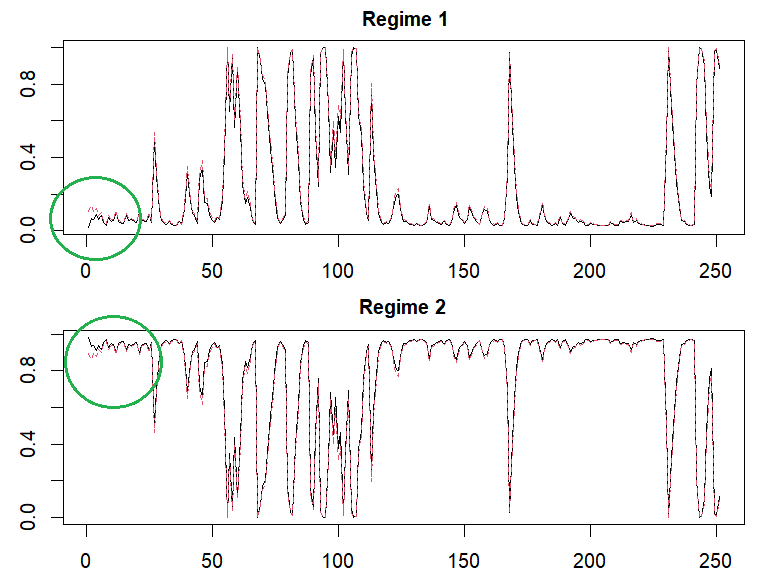
# draw filtered probabilities of two states
x11(); par(mfrow=c(2,1))
matplot(cbind(rsm@Fit@filtProb[,1],hf$fp[,2]),
main = “Regime 1”, type=“l”, cex.main=1)
matplot(cbind(rsm@Fit@filtProb[,2],hf$fp[,1]),
main = “Regime 2”, type=“l”, cex.main=1)
# comparison of parameters
invisible(print(“—–Comparison of two results—–“))
invisible(print(“constant and beta1”))
cbind(rsm@Coef, cbind(mle$par[1:2],mle$par[3:4]))
invisible(print(“sigma”))
cbind(rsm@std, mle$par[5:6])
invisible(print(“p00, 011”))
cbind(diag(rsm@transMat), 1/(1+exp(–mle$par[7:8])))
invisible(print(“loglikelihood”))
cbind(rsm@Fit@logLikel, mle$value)

Concluding Remarks
In this post, we explains Hamilton regime switching model by taking AR(1) model as an example and implement R code without the help of MSwM R package. Smoothed probabilities as well as filtered probabilities are important since it use all information. In the next post, we will implement smoothed probabilities with some detail derivations. \(\blacksquare\) var vglnk = {key: '949efb41171ac6ec1bf7f206d57e90b8'}; (function(d, t) { var s = d.createElement(t); s.type = 'text/javascript'; s.async = true;// s.defer = true;// s.src = '//cdn.viglink.com/api/vglnk.js'; s.src = 'https://www.r-bloggers.com/wp-content/uploads/2020/08/vglnk.js'; var r = d.getElementsByTagName(t)[0]; r.parentNode.insertBefore(s, r); }(document, 'script'));To leave a comment for the author, please follow the link and comment on their blog: K & L Fintech Modeling.
R-bloggers.com offers daily e-mail updates about R news and tutorials about learning R and many other topics. Click here if you're looking to post or find an R/data-science job.
Want to share your content on R-bloggers? click here if you have a blog, or here if you don't.