The Gowers uniformity norm of order 1+

What's new 2021-07-25

In the modern theory of higher order Fourier analysis, a key role are played by the Gowers uniformity norms ${\| \|_{U^k}}$ for ${k=1,2,\dots}$ . For finitely supported functions ${f: {\bf Z} \rightarrow {\bf C}}$ , one can define the (non-normalised) Gowers norm ${\|f\|_{\tilde U^k({\bf Z})}}$ by the formula

$\displaystyle \|f\|_{\tilde U^k({\bf Z})}^{2^k} := \sum_{n,h_1,\dots,h_k \in {\bf Z}} \prod_{\omega_1,\dots,\omega_k \in \{0,1\}} {\mathcal C}^{\omega_1+\dots+\omega_k} f(x+\omega_1 h_1 + \dots + \omega_k h_k)$

where ${{\mathcal C}}$ denotes complex conjugation, and then on any discrete interval ${[N] = \{1,\dots,N\}}$ and any function ${f: [N] \rightarrow {\bf C}}$ we can then define the (normalised) Gowers norm

$\displaystyle \|f\|_{U^k([N])} := \| f 1_{[N]} \|_{\tilde U^k({\bf Z})} / \|1_{[N]} \|_{\tilde U^k({\bf Z})}$

where ${f 1_{[N]}: {\bf Z} \rightarrow {\bf C}}$ is the extension of ${f}$ by zero to all of ${{\bf Z}}$ . Thus for instance

$\displaystyle \|f\|_{U^1([N])} = |\mathop{\bf E}_{n \in [N]} f(n)|$

(which technically makes ${\| \|_{U^1([N])}}$ a seminorm rather than a norm), and one can calculate

$\displaystyle \|f\|_{U^2([N])} \asymp (N \int_0^1 |\mathop{\bf E}_{n \in [N]} f(n) e(-\alpha n)|^4\ d\alpha)^{1/4} \ \ \ \ \ (1)$

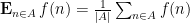where ${e(\theta) := e^{2\pi i \alpha}}$ , and we use the averaging notation ${\mathop{\bf E}_{n \in A} f(n) = \frac{1}{|A|} \sum_{n \in A} f(n)}$ .

The significance of the Gowers norms is that they control other multilinear forms that show up in additive combinatorics. Given any polynomials ${P_1,\dots,P_m: {\bf Z}^d \rightarrow {\bf Z}}$ and functions ${f_1,\dots,f_m: [N] \rightarrow {\bf C}}$ , we define the multilinear form

$\displaystyle \Lambda^{P_1,\dots,P_m}(f_1,\dots,f_m) := \sum_{n \in {\bf Z}^d} \prod_{j=1}^m f 1_{[N]}(P_j(n)) / \sum_{n \in {\bf Z}^d} \prod_{j=1}^m 1_{[N]}(P_j(n))$

(assuming that the denominator is finite and non-zero). Thus for instance

$\displaystyle \Lambda^{\mathrm{n}}(f) = \mathop{\bf E}_{n \in [N]} f(n)$

$\displaystyle \Lambda^{\mathrm{n}, \mathrm{n}+\mathrm{r}}(f,g) = (\mathop{\bf E}_{n \in [N]} f(n)) (\mathop{\bf E}_{n \in [N]} g(n))$

$\displaystyle \Lambda^{\mathrm{n}, \mathrm{n}+\mathrm{r}, \mathrm{n}+2\mathrm{r}}(f,g,h) \asymp \mathop{\bf E}_{n \in [N]} \mathop{\bf E}_{r \in [-N,N]} f(n) g(n+r) h(n+2r)$

$\displaystyle \Lambda^{\mathrm{n}, \mathrm{n}+\mathrm{r}, \mathrm{n}+\mathrm{r}^2}(f,g,h) \asymp \mathop{\bf E}_{n \in [N]} \mathop{\bf E}_{r \in [-N^{1/2},N^{1/2}]} f(n) g(n+r) h(n+r^2)$

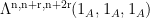where we view ${\mathrm{n}, \mathrm{r}}$ as formal (indeterminate) variables, and ${f,g,h: [N] \rightarrow {\bf C}}$ are understood to be extended by zero to all of ${{\bf Z}}$ . These forms are used to count patterns in various sets; for instance, the quantity ${\Lambda^{\mathrm{n}, \mathrm{n}+\mathrm{r}, \mathrm{n}+2\mathrm{r}}(1_A,1_A,1_A)}$ is closely related to the number of length three arithmetic progressions contained in ${A}$ . Let us informally say that a form ${\Lambda^{P_1,\dots,P_m}(f_1,\dots,f_m)}$ is controlled by the ${U^k[N]}$ norm if the form is small whenever ${f_1,\dots,f_m: [N] \rightarrow {\bf C}}$ are ${1}$ -bounded functions with at least one of the ${f_j}$ small in ${U^k[N]}$ norm. This definition was made more precise by Gowers and Wolf, who then defined the true complexity of a form ${\Lambda^{P_1,\dots,P_m}}$ to be the least ${s}$ such that ${\Lambda^{P_1,\dots,P_m}}$ is controlled by the ${U^{s+1}[N]}$ norm. For instance,

${\Lambda^{\mathrm{n}}}$ and ${\Lambda^{\mathrm{n}, \mathrm{n} + \mathrm{r}}}$ have true complexity ${0}$ ;
${\Lambda^{\mathrm{n}, \mathrm{n} + \mathrm{r}, \mathrm{n} + \mathrm{2r}}}$ has true complexity ${1}$ ;
${\Lambda^{\mathrm{n}, \mathrm{n} + \mathrm{r}, \mathrm{n} + \mathrm{2r}, \mathrm{n} + \mathrm{3r}}}$ has true complexity ${2}$ ;
The form ${\Lambda^{\mathrm{n}, \mathrm{n}+2}}$ (which among other things could be used to count twin primes) has infinite true complexity (which is quite unfortunate for applications).

Roughly speaking, patterns of complexity ${1}$ or less are amenable to being studied by classical Fourier analytic tools (the Hardy-Littlewood circle method); patterns of higher complexity can be handled (in principle, at least) by the methods of higher order Fourier analysis; and patterns of infinite complexity are out of range of both methods and are generally quite difficult to study. See these recent slides of myself for some further discussion.

Gowers and Wolf formulated a conjecture on what this complexity should be, at least for linear polynomials ${P_1,\dots,P_m}$ ; Ben Green and I thought we had resolved this conjecture back in 2010, though it turned out there was a subtle gap in our arguments and we were only able to resolve the conjecture in a partial range of cases. However, the full conjecture was recently resolved by Daniel Altman.

The ${U^1}$ (semi-)norm is so weak that it barely controls any averages at all. For instance the average

$\displaystyle \Lambda^{2\mathrm{n}}(f) = \mathop{\bf E}_{n \in [N], \hbox{ even}} f(n)$

is not controlled by the ${U^1[N]}$ semi-norm: it is perfectly possible for a ${1}$ -bounded function ${f: [N] \rightarrow {\bf C}}$ to even have vanishing ${U^1([N])}$ norm but have large value of ${\Lambda^{2\mathrm{n}}(f)}$ (consider for instance the parity function ${f(n) := (-1)^n}$ ).

Because of this, I propose inserting an additional norm in the Gowers uniformity norm hierarchy between the ${U^1}$ and ${U^2}$ norms, which I will call the ${U^{1^+}}$ (or “profinite ${U^1}$ “) norm:

$\displaystyle \| f\|_{U^{1^+}[N]} := \frac{1}{N} \sup_P |\sum_{n \in P} f(n)| = \sup_P | \mathop{\bf E}_{n \in [N]} f 1_P(n)|$

where ${P}$ ranges over all arithmetic progressions in ${[N]}$ . This can easily be seen to be a norm on functions ${f: [N] \rightarrow {\bf C}}$ that controls the ${U^1[N]}$ norm. It is also basically controlled by the ${U^2[N]}$ norm for ${1}$ -bounded functions ${f}$ ; indeed, if ${P}$ is an arithmetic progression in ${[N]}$ of some spacing ${q \geq 1}$ , and if ${\psi}$ be a standard bump function supported on ${[-1,1]}$ with total mass and ${\delta>0}$ is a parameter then

$\displaystyle \mathop{\bf E}_{n \in [N]} f 1_P(n) \ll |\mathop{\bf E}_{n \in [N]; h, k \in [-N,N]} \frac{1}{\delta} \psi(\frac{h}{\delta N}) 1_{q|h} 1_P(n+k) f(n+h+k)| + \delta$

which after some Fourier expansion of ${\delta \psi(\frac{h}{\delta N}) 1_{r|h}}$ gives

$\displaystyle \mathop{\bf E}_{n \in [N]} f 1_P(n) \ll \frac{1}{\delta} \sup_\alpha |\mathop{\bf E}_{n \in [N]; h, k \in [-N,N]} e(\alpha h) 1_P(n+k) f(n+h+k)| + \delta.$

Writing ${e(\alpha h) = e(\alpha(n+h)) e(-\alpha n)}$ and using the Gowers–Cauchy–Schwarz inequality, we conclude

$\displaystyle \mathop{\bf E}_{n \in [N]} f 1_P(n) \ll \frac{1}{\delta} \|f\|_{U^2([N])} + \delta$

hence on optimising in ${\delta}$ we have

$\displaystyle \| f\|_{U^{1^+}[N]} \ll \|f\|_{U^2[N]}^{1/2}.$

Forms which are controlled by the ${U^{1^+}}$ norm (but not ${U^1}$ ) would then have their true complexity adjusted to ${0^+}$ with this insertion.

The ${U^{1^+}}$ norm recently appeared implicitly in work of Peluse and Prendiville, who showed that the form ${\Lambda^{\mathrm{n}, \mathrm{n}+\mathrm{r}, \mathrm{n}+\mathrm{r}^2}(f,g,h)}$ had true complexity ${0^+}$ in this notation (with polynomially strong bounds). [Actually, strictly speaking this control was only shown for the third function ${h}$ ; for the first two functions ${f,g}$ one needs to localize the ${U^{1^+}}$ norm to intervals of length ${\sim \sqrt{N}}$ . But I will ignore this technical point to keep the exposition simple.] The weaker claim that ${\Lambda^{\mathrm{n}, \mathrm{n}+\mathrm{r}^2}(f,g)}$ has true complexity ${0^+}$ is substantially easier to prove (one can apply the circle method together with Gauss sum estimates).

The well known inverse theorem for the ${U^2}$ norm tells us that if a ${1}$ -bounded function ${f}$ has ${U^2[N]}$ norm at least ${\eta}$ for some ${0 < \eta < 1}$ , then there is a Fourier phase ${n \mapsto e(\alpha n)}$ such that

$\displaystyle |\mathop{\bf E}_{n \in [N]} f(n) e(-\alpha n)| \gg \eta^2;$

this follows easily from (1) and Plancherel’s theorem. Conversely, from the Gowers–Cauchy–Schwarz inequality one has

$\displaystyle |\mathop{\bf E}_{n \in [N]} f(n) e(-\alpha n)| \ll \|f\|_{U^2[N]}.$

For ${U^1[N]}$ one has a trivial inverse theorem; by definition, the ${U^1[N]}$ norm of ${f}$ is at least ${\eta}$ if and only if

$\displaystyle |\mathop{\bf E}_{n \in [N]} f(n)| \geq \eta.$

Thus the frequency ${\alpha}$ appearing in the ${U^2}$ inverse theorem can be taken to be zero when working instead with the ${U^1}$ norm.

For ${U^{1^+}}$ one has the intermediate situation in which the frequency ${\alpha}$ is not taken to be zero, but is instead major arc. Indeed, suppose that ${f}$ is ${1}$ -bounded with ${\|f\|_{U^{1^+}[N]} \geq \eta}$ , thus

$\displaystyle |\mathop{\bf E}_{n \in [N]} 1_P(n) f(n)| \geq \eta$

for some progression ${P}$ . This forces the spacing ${q}$ of this progression to be ${\ll 1/\eta}$ . We write the above inequality as

$\displaystyle |\mathop{\bf E}_{n \in [N]} 1_{n=b\ (q)} 1_I(n) f(n)| \geq \eta$

for some residue class ${b\ (q)}$ and some interval ${I}$ . By Fourier expansion and the triangle inequality we then have

$\displaystyle |\mathop{\bf E}_{n \in [N]} e(-an/q) 1_I(n) f(n)| \geq \eta$

for some integer ${a}$ . Convolving ${1_I}$ by ${\psi_\delta: n \mapsto \frac{1}{\delta} \psi(n/\delta)}$ for ${\delta}$ a small multiple of ${\eta}$ and ${\psi}$ a Schwartz function of unit mass with Fourier transform supported on ${[-1,1]}$ , we have

$\displaystyle |\mathop{\bf E}_{n \in [N]} e(-an/q) (1_I * \psi_\delta)(n) f(n)| \gg \eta.$

The Fourier transform of ${1_I * \psi_\delta}$ is bounded and supported on ${[-1/\delta,1/\delta]}$ , thus by Fourier expansion and the triangle inequality we have

$\displaystyle |\mathop{\bf E}_{n \in [N]} e(-an/q) e(-\xi n) f(n)| \gg \eta$

for some ${\xi \in [-1/\delta,1/\delta]}$ , so in particular ${\xi = O(1/\eta)}$ . Thus we have

$\displaystyle |\mathop{\bf E}_{n \in [N]} f(n) e(-\alpha n)| \gg \eta \ \ \ \ \ (2)$

for some ${\alpha}$ of the major arc form ${\alpha = \frac{a}{q} + O(1/\eta)}$ with ${1 \leq q \leq 1/\eta}$ . Conversely, for ${\alpha}$ of this form, some routine summation by parts gives the bound

$\displaystyle |\mathop{\bf E}_{n \in [N]} f(n) e(-\alpha n)| \ll \frac{q}{\eta} \|f\|_{U^{1^+}[N]} \ll \frac{1}{\eta^2} \|f\|_{U^{1^+}[N]}$

so if (2) holds for a ${1}$ -bounded ${f}$ then one must have ${\|f\|_{U^{1^+}[N]} \gg \eta^3}$ .

Here is a diagram showing some of the control relationships between various Gowers norms, multilinear forms, and duals of classes ${{\mathcal F}}$ of functions (where each class of functions ${{\mathcal F}}$ induces a dual norm ${\| f \|_{{\mathcal F}^*} := \sup_{\phi \in {\mathcal F}} \mathop{\bf E}_{n \in[N]} f(n) \overline{\phi(n)}}$ :

The Gowers norms have counterparts for measure-preserving systems ${(X,T,\mu)}$ , known as Host-Kra seminorms. The ${U^1(X)}$ norm can be defined for ${f \in L^\infty(X)}$ as

$\displaystyle \|f\|_{U^1(X)} := \lim_{N \rightarrow \infty} \int_X |\mathop{\bf E}_{n \in [N]} T^n f|\ d\mu$

and the ${U^2}$ norm can be defined as

$\displaystyle \|f\|_{U^2(X)}^4 := \lim_{N \rightarrow \infty} \mathop{\bf E}_{n \in [N]} \| T^n f \overline{f} \|_{U^1(X)}^2.$

The ${U^1(X)}$ seminorm is orthogonal to the invariant factor ${Z^0(X)}$ (generated by the (almost everywhere) invariant measurable subsets of ${X}$ ) in the sense that a function ${f \in L^\infty(X)}$ has vanishing ${U^1(X)}$ seminorm if and only if it is orthogonal to all ${Z^0(X)}$ -measurable (bounded) functions. Similarly, the ${U^2(X)}$ norm is orthogonal to the Kronecker factor ${Z^1(X)}$ , generated by the eigenfunctions of ${X}$ (that is to say, those ${f}$ obeying an identity ${Tf = \lambda f}$ for some ${T}$ -invariant ${\lambda}$ ); for ergodic systems, it is the largest factor isomorphic to rotation on a compact abelian group. In analogy to the Gowers ${U^{1^+}[N]}$ norm, one can then define the Host-Kra ${U^{1^+}(X)}$ seminorm by

$\displaystyle \|f\|_{U^{1^+}(X)} := \sup_{q \geq 1} \frac{1}{q} \lim_{N \rightarrow \infty} \int_X |\mathop{\bf E}_{n \in [N]} T^{qn} f|\ d\mu;$

it is orthogonal to the profinite factor ${Z^{0^+}(X)}$ , generated by the periodic sets of ${X}$ (or equivalently, by those eigenfunctions whose eigenvalue is a root of unity); for ergodic systems, it is the largest factor isomorphic to rotation on a profinite abelian group.