Venn and Euler type diagrams for vector spaces and abelian groups

What's new 2021-11-08

A popular way to visualise relationships between some finite number of sets is via Venn diagrams, or more generally Euler diagrams. In these diagrams, a set is depicted as a two-dimensional shape such as a disk or a rectangle, and the various Boolean relationships between these sets (e.g., that one set is contained in another, or that the intersection of two of the sets is equal to a third) is represented by the Boolean algebra of these shapes; Venn diagrams correspond to the case where the sets are in “general position” in the sense that all non-trivial Boolean combinations of the sets are non-empty. For instance to depict the general situation of two sets ${A,B}$ together with their intersection ${A \cap B}$ and ${A \cup B}$ one might use a Venn diagram such as

venn

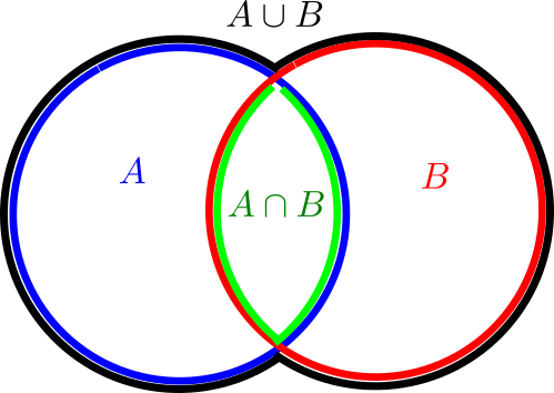
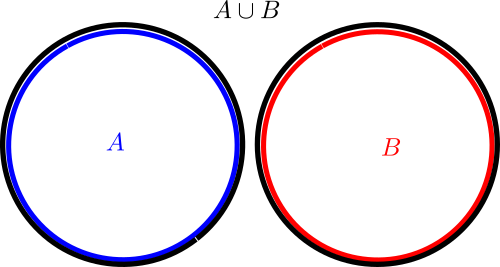
(where we have given each region depicted a different color, and moved the edges of each region a little away from each other in order to make them all visible separately), but if one wanted to instead depict a situation in which the intersection ${A \cap B}$ was empty, one could use an Euler diagram such as

euler

One can use the area of various regions in a Venn or Euler diagram as a heuristic proxy for the cardinality ${|A|}$ (or measure ${\mu(A)}$ ) of the set ${A}$ corresponding to such a region. For instance, the above Venn diagram can be used to intuitively justify the inclusion-exclusion formula

$\displaystyle |A \cup B| = |A| + |B| - |A \cap B|$

for finite sets ${A,B}$ , while the above Euler diagram similarly justifies the special case

$\displaystyle |A \cup B| = |A| + |B|$

for finite disjoint sets ${A,B}$ .

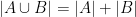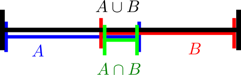
While Venn and Euler diagrams are traditionally two-dimensional in nature, there is nothing preventing one from using one-dimensional diagrams such as

venn1d

or even three-dimensional diagrams such as this one from Wikipedia:

venn-3d

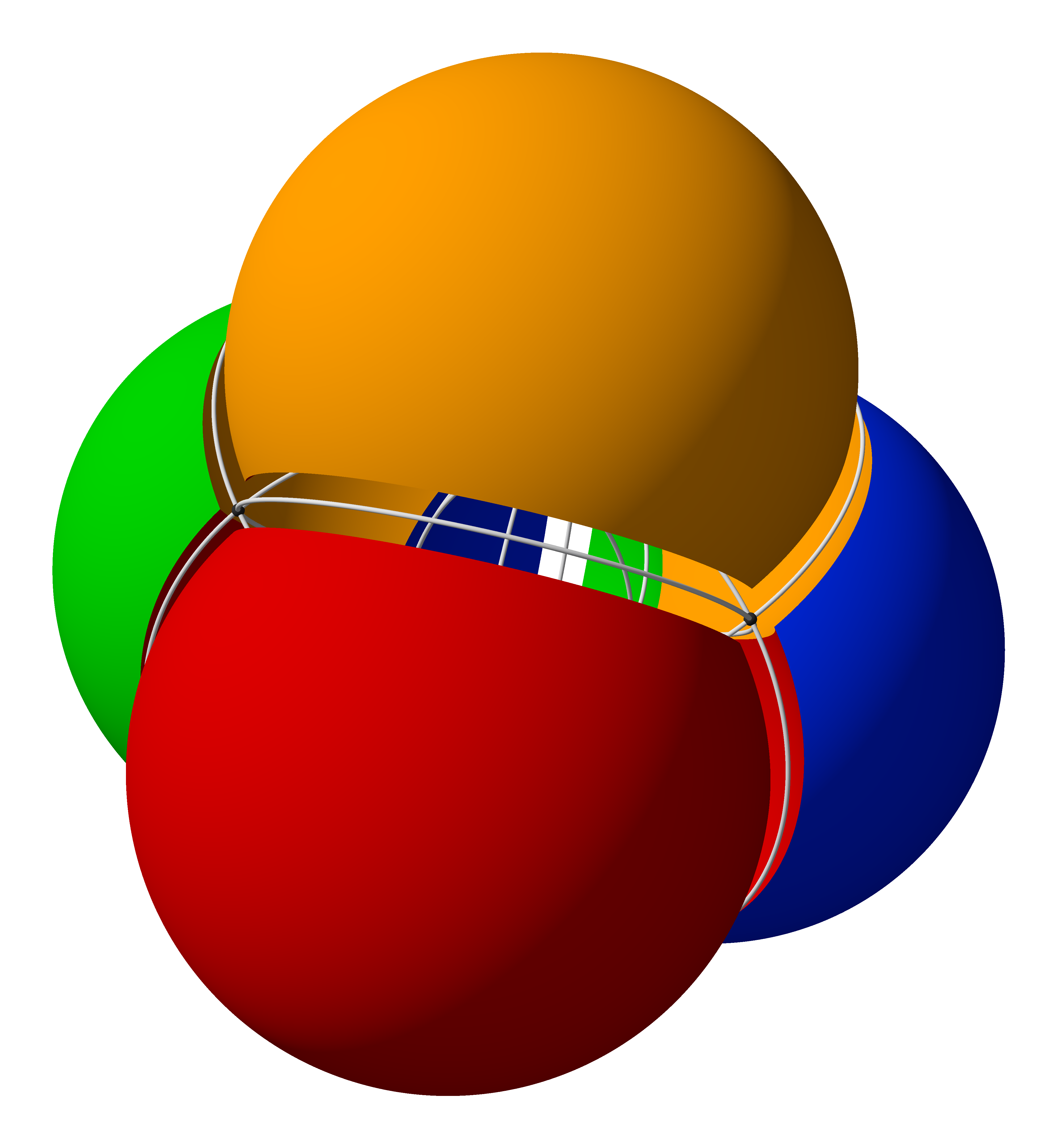
Of course, in such cases one would use length or volume as a heuristic proxy for cardinality or measure, rather than area.

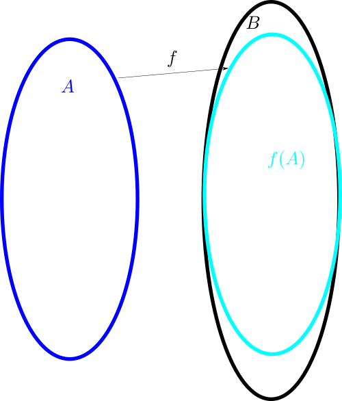
With the addition of arrows, Venn and Euler diagrams can also accommodate (to some extent) functions between sets. Here for instance is a depiction of a function ${f: A \rightarrow B}$ , the image ${f(A)}$ of that function, and the image ${f(A')}$ of some subset ${A'}$ of ${A}$ :

afb

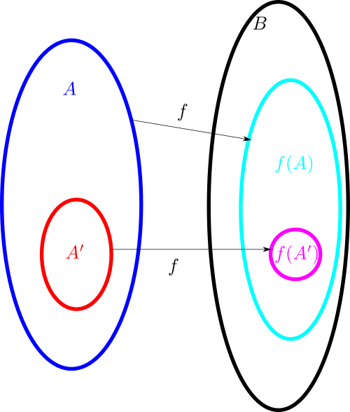
Here one can illustrate surjectivity of ${f: A \rightarrow B}$ by having ${f(A)}$ fill out all of ${B}$ ; one can similarly illustrate injectivity of ${f}$ by giving ${f(A)}$ exactly the same shape (or at least the same area) as ${A}$ . So here for instance might be how one would illustrate an injective function ${f: A \rightarrow B}$ :

afb-injective

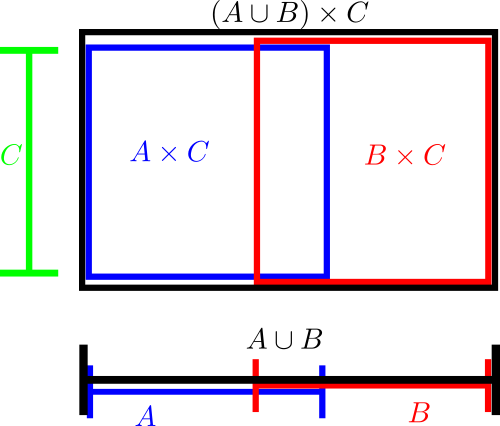
Cartesian product operations can be incorporated into these diagrams by appropriate combinations of one-dimensional and two-dimensional diagrams. Here for instance is a diagram that illustrates the identity ${(A \cup B) \times C = (A \times C) \cup (B \times C)}$ :

cartesian

In this blog post I would like to propose a similar family of diagrams to illustrate relationships between vector spaces (over a fixed base field ${k}$ , such as the reals) or abelian groups, rather than sets. The categories of ( ${k}$ -)vector spaces and abelian groups are quite similar in many ways; the former consists of modules over a base field ${k}$ , while the latter consists of modules over the integers ${{\bf Z}}$ ; also, both categories are basic examples of abelian categories. The notion of a dimension in a vector space is analogous in many ways to that of cardinality of a set; see this previous post for an instance of this analogy (in the context of Shannon entropy).

As with Venn and Euler diagrams, the diagrams I propose for vector spaces (or abelian groups) can be set up in any dimension. For simplicity, let’s begin with one dimension, and restrict attention to vector spaces (the situation for abelian groups is basically identical). In this one-dimensional model we will be able to depict the following relations and operations between vector spaces:

The inclusion ${W \leq V}$ of one vector space ${V}$ in another ${W}$ (here I prefer to use the group notation ${\leq}$ for inclusion rather than the set notation ${\subseteq}$ ).
The quotient ${V/W}$ of a vector space ${V}$ by a subspace ${W}$ .
A linear transformation ${T: V \rightarrow W}$ between vector spaces, as well as the kernel ${\mathrm{ker}(T)}$ , image ${\mathrm{im}(T)}$ , cokernel ${\mathrm{coker}(T) = W/\mathrm{im}(T)}$ , and the coimage ${\mathrm{coim}(T) = V/\mathrm{ker}(T)}$ .
A single short or long exact sequence between vector spaces.
(A heuristic proxy for) the dimension of a vector space.
Direct sum ${V \otimes W}$ of two spaces.

The idea is to use half-open intervals ${[a,b)}$ in the real line for any ${a<b}$ to model vector spaces. In fact we can make an explicit correspondence: let us identify each half-open interval ${[a,b)}$ with the (infinite-dimensional) vector space

$\displaystyle [a,b) \equiv \{ f \in C([a,b]): f(b) = 0 \},$

that is ${[a,b)}$ is identified with the space of continuous functions ${f:[a,b] \rightarrow {\bf R}}$ on the interval ${[a,b]}$ that vanish at the right-endpoint ${b}$ . Such functions can be continuously extended by zero to the half-line ${[a,+\infty)}$ .

Note that if ${a < b < c}$ then the vector space ${[a,b)}$ is a subspace of ${[a,c)}$ , if we extend the functions in both spaces by zero to the half-line ${[a,+\infty)}$ ; furthermore, the quotient of ${[a,c)}$ by ${[a,b)}$ is naturally identifiable with ${[b,c)}$ . Thus, an inclusion ${W \leq V}$ , as well as the quotient space ${V/W}$ , can be modeled here as follows:

coker

In contrast, if ${a < b < c < d}$ , it is significantly less “natural” to view ${[b,c)}$ as a subspace of ${[a,d)}$ ; one could do it by extending functions in ${[b,c)}$ to the right by zero and to the left by constants, but in this notational convention one should view such an identification as “artificial” and to be avoided.

All of the spaces ${[a,b)}$ are infinite dimensional, but morally speaking the dimension of the vector space ${[a,b)}$ is “proportional” to the length ${b-a}$ of the corresponding interval. Intuitively, if we try to discretise this vector space by sampling at some mesh of spacing ${\varepsilon}$ , one gets a finite-dimensional vector space of dimension roughly ${(b-a)/\varepsilon}$ . Already the above diagram now depicts the basic identity

$\displaystyle \mathrm{dim}(V) = \mathrm{dim}(W) + \mathrm{dim}(V/W)$

between a finite-dimensional vector space ${V}$ , a subspace ${W}$ of that space, and a quotient of that space.

Note that if ${a < b < c < d}$ , then there is a linear transformation ${T}$ from the vector space ${[a,c)}$ to the vector space ${[b,d)}$ which takes a function ${f}$ in ${[a,c)}$ , restricts it to ${[b,c)}$ , then extends it by zero to ${[b,d)}$ . The kernel of this transformation is ${[a,b)}$ , the image is (isomorphic to) ${[b,c)}$ , the cokernel is (isomorphic to) ${[c,d)}$ , and the coimage is (isomorphic to) ${[b,c)}$ . With this in mind, we can now depict a general linear transformation ${T: V \rightarrow W}$ and its associated spaces by the following diagram:

rank-nullity

Note how the first isomorphism theorem and the rank-nullity theorem are heuristically illustrated by this diagram. One can specialise to the case of injective, surjective, or bijective transformations ${T}$ by degenerating one or more of the half-open intervals in the above diagram to the empty interval. A left shift on ${[a,b)}$ gives rise to a nilpotent linear transformation ${T}$ from ${[a,b)}$ to itself:

nilpotent

In a similar spirit, a short exact sequence ${0 \rightarrow U \rightarrow V \rightarrow W \rightarrow 0}$ of vector spaces (or abelian groups) can now be depicted by the diagram

short-exact

and a long exact sequence ${V_1 \rightarrow V_2 \rightarrow V_3 \rightarrow \dots}$ can similarly be depicted by the diagram

long-exact

where we have omitted the arrows for brevity.

One can associate the disjoint union of half-open intervals to the direct sum of the associated vector spaces, giving a way to depict direct sums via this notation:

direct-sum

To increase the expressiveness of this notation we now move to two dimensions, where we can also depict the following additional relations and operations:

The intersection ${U \cap V}$ and sum ${U+V}$ of two subspaces ${U,V \leq W}$ of an ambient space ${W}$ ;
Multiple short or long exact sequences;
The tensor product ${U \otimes V}$ of two vector spaces ${U,V}$ .

Here, we replace half-open intervals by half-open sets: geometric shapes ${S}$ , such as polygons or disks, which contain some portion of the boundary (drawn using solid lines) but omit some other portion of the boundary (drawn with dashed lines). Each such shape can be associated with a vector space, namely the continuous functions on ${\overline{S}}$ that vanish on the omitted portion of the boundary. All of the relations that were previously depicted using one-dimensional diagrams can now be similarly depicted using two-dimensional diagrams. For instance, here is a two-dimensional depiction of a vector space ${V}$ , a subspace ${W}$ , and its quotient ${V/W}$ :

coker-2D

(In this post I will try to consistently make the lower and left boundaries of these regions closed, and the upper and right boundaries open, although this is not essential for this notation to be applicable.)

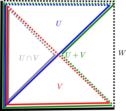
But now we can depict some additional relations. Here for instance is one way to depict the intersection ${U \cap V}$ and sum ${U+V}$ of two subspaces ${U,V \leq W}$ :

uvw

Note how this illustrates the identity

$\displaystyle \mathrm{dim}(U + V) = \mathrm{dim}(U) + \mathrm{dim}(V) - \mathrm{dim}(U \cap V)$

between finite-dimensional vector spaces ${U, V}$ , as well as some standard isomorphisms such as ${(U+V)/U \equiv V/(U \cap V)}$ .

Two finite subgroups ${H,K}$ of an abelian group ${G}$ are said to be commensurable if ${H \cap K}$ is a finite index subgroup of ${H+K}$ . One can depict this by making the area of the region between ${H \cap K}$ and ${H+K}$ small and/or colored with some specific color:

ghk

Here the commensurability of ${H,K}$ is equivalent to the finiteness of the groups ${H / (H \cap K) \equiv (H+K)/K}$ and ${K / (H \cap K) \equiv (H+K)/H}$ , which correspond to the gray triangles in the above diagram. Now for instance it becomes intuitively clear why commensurability should be an equivalence relation.

To illustrate how this notation can support multiple short exact sequences, I gave myself the exercise of using this notation to depict the snake lemma, as labeled by this following diagram taken from the just linked Wikipedia page:

snake

This turned out to be remarkably tricky to accomplish without introducing degeneracies (e.g., one of the kernels or cokernels vanishing). Here is one solution I came up with; perhaps there are more elegant ones. In particular, there should be a depiction that more explicitly captures the duality symmetry of the snake diagram.

bigsnake

Here, the maps between the six spaces 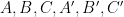${A,B,C,A',B',C'}$ are the obvious restriction maps (and one can visually verify that the two squares in the snake diagram actually commute). Each of the kernel and cokernel spaces of the three vertical restriction maps ${a,b,c}$ are then associated to the union of two of the subregions as indicated in the diagram.

With our notation, the (algebraic) tensor product of an interval ${[a,b)}$ and another interval ${[c,d)}$ is not quite ${[a,b) \times [c,d)}$ , but this becomes true if one uses the ${C^*}$ -algebra version of the tensor product, thanks to the Stone-Weierstrass theorem. So one can plausibly use Cartesian products as a proxy for the vector space tensor product. For instance, here is a depiction of the relation ${(U \otimes W) / (V \otimes W) \equiv (U/V) \otimes W}$ when ${V}$ is a subspace of ${U}$ :

tensor-quotient

There are unfortunately some limitations to this notation: for instance, no matter how many dimensions one uses for one’s diagrams, these diagrams would suggest the incorrect identity

$\displaystyle \mathrm{dim}(U +V + W) = \mathrm{dim} U + \mathrm{dim} V + \mathrm{dim} W - \mathrm{dim} (U \cap V) - \mathrm{dim} (U \cap W) - \mathrm{dim} (V \cap W) + \mathrm{dim}(U \cap V \cap W),$

(which incidentally is, at this time of writing, the highest-voted answer to the MathOverflow question “Examples of common false beliefs in mathematics“). (See also this previous blog post for a similar phenomenon when using sets or vector spaces to model entropy of information variables.) Nevertheless it seems accurate enough to be of use in illustrating many common relations between vector spaces and abelian groups. With appropriate grains of salt it might also be usable for further categories beyond these two, though for non-abelian categories one should proceed with caution, as the diagram may suggest relations that are not actually true in this category. For instance, in the category of topological groups one might use the diagram

topgroup

to describe the fact that an arbitrary topological group splits into a connected subgroup and a totally disconnected quotient, or in the category of finite-dimensional Lie algebras over the reals one might use the diagram

liealg

to describe the fact that such algebras split into the solvable radical and a semisimple quotient.