Partially specified mathematical objects, ambient parameters, and asymptotic notation

What's new 2022-05-11

In orthodox first-order logic, variables and expressions are only allowed to take one value at a time; a variable ${x}$ , for instance, is not allowed to equal ${+3}$ and ${-3}$ simultaneously. We will call such variables completely specified. If one really wants to deal with multiple values of objects simultaneously, one is encouraged to use the language of set theory and/or logical quantifiers to do so.

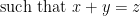
However, the ability to allow expressions to become only partially specified is undeniably convenient, and also rather intuitive. A classic example here is that of the quadratic formula:

$\displaystyle \hbox{If } x,a,b,c \in {\bf R} \hbox{ with } a \neq 0, \hbox{ then }$

$\displaystyle ax^2+bx+c=0 \hbox{ if and only if } x = \frac{-b \pm \sqrt{b^2-4ac}}{2a}. \ \ \ \ \ (1)$

Strictly speaking, the expression ${x = \frac{-b \pm \sqrt{b^2-4ac}}{2a}}$ is not well-formed according to the grammar of first-order logic; one should instead use something like

$\displaystyle x = \frac{-b - \sqrt{b^2-4ac}}{2a} \hbox{ or } x = \frac{-b + \sqrt{b^2-4ac}}{2a}$

$\displaystyle x \in \left\{ \frac{-b - \sqrt{b^2-4ac}}{2a}, \frac{-b + \sqrt{b^2-4ac}}{2a} \right\}$

$\displaystyle x = \frac{-b + \epsilon \sqrt{b^2-4ac}}{2a} \hbox{ for some } \epsilon \in \{-1,+1\}$

in order to strictly adhere to this grammar. But none of these three reformulations are as compact or as conceptually clear as the original one. In a similar spirit, a mathematical English sentence such as

$\displaystyle \hbox{The sum of two odd numbers is an even number} \ \ \ \ \ (2)$

is also not a first-order sentence; one would instead have to write something like

$\displaystyle \hbox{For all odd numbers } x, y, \hbox{ the number } x+y \hbox{ is even} \ \ \ \ \ (3)$

$\displaystyle \hbox{For all odd numbers } x,y \hbox{ there exists an even number } z \ \ \ \ \ (4)$

$\displaystyle \hbox{ such that } x+y=z$

instead. These reformulations are not all that hard to decipher, but they do have the aesthetically displeasing effect of cluttering an argument with temporary variables such as ${x,y,z}$ which are used once and then discarded.

Another example of partially specified notation is the innocuous ${\ldots}$ notation. For instance, the assertion

$\displaystyle \pi=3.14\ldots,$

when written formally using first-order logic, would become something like

$\displaystyle \pi = 3 + \frac{1}{10} + \frac{4}{10^2} + \sum_{n=3}^\infty \frac{a_n}{10^n} \hbox{ for some sequence } (a_n)_{n=3}^\infty$

$\displaystyle \hbox{ with } a_n \in \{0,1,2,3,4,5,6,7,8,9\} \hbox{ for all } n,$

which is not exactly an elegant reformulation. Similarly with statements such as

$\displaystyle \tan x = x + \frac{x^3}{3} + \ldots \hbox{ for } |x| < \pi/2$

$\displaystyle \tan x = x + \frac{x^3}{3} + O(|x|^5) \hbox{ for } |x| < \pi/2.$

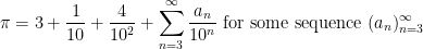
Below the fold I’ll try to assign a formal meaning to partially specified expressions such as (1), for instance allowing one to condense (2), (3), (4) to just

$\displaystyle \hbox{odd} + \hbox{odd} = \hbox{even}.$

When combined with another common (but often implicit) extension of first-order logic, namely the ability to reason using ambient parameters, we become able to formally introduce asymptotic notation such as the big-O notation ${O()}$ or the little-o notation ${o()}$ . We will explain how to do this at the end of this post.

— 1. Partially specified objects —

Let’s try to assign a formal meaning to partially specified mathematical expressions. We now allow expressions ${X}$ to not necessarily be a single (completely specified) mathematical object, but more generally an partially specified instance of a class ${\{X\}}$ of mathematical objects. For instance, ${\pm 3}$ denotes a partially specified instance of the class ${\{ \pm 3 \} = \{ 3, -3\}}$ of numbers consisting of ${3}$ and ${-3}$ ; that is to say, a number which is either ${-3}$ and ${+3}$ . A single completely specified mathematical object, such as the number ${3}$ , can now be also interpreted as the (unique) instance of a class ${\{ 3 \}}$ consisting only of ${3}$ . Here we are using set notation to describe classes, ignoring for now the well known issue from Russell’s paradox that some extremely large classes are technically not sets, as this is not the main focus of our discussion here.

For reasons that will become clearer later, we will use the symbol ${==}$ rather than ${=}$ to denote the assertion that two partially specified objects range across exactly the same class. That is to say, we use ${X==Y}$ as a synonym for ${\{X\} = \{Y\}}$ . Thus, for instance, it is not the case that ${3 == \pm 3}$ , because the there are class ${\{\pm 3\}}$ has instances that ${\{3\}}$ does not.

Any finite sequence ${x_1,\dots,x_n}$ of objects can also be viewed as a partially specified instances of a class ${\{x_1,\dots,x_n\}}$ , which I will denote ${x_1|\dots|x_n}$ in analogy with regular expressions, thus we now also have a new name ${\{x_1|\dots|x_n\}}$ for the set ${\{x_1,\dots,x_n\}}$ . (One could in fact propose ${x_1,\dots,x_n}$ as the notation for ${x_1|\dots|x_n}$ , as is done implicitly in assertions such as “ ${P(n)}$ is true for ${n=1,2,3}$ “, but this creates notational conflicts with other uses of the comma in mathematics, such as the notation ${(x_1,\dots,x_n)}$ for an ${n}$ -tuple, so I will use the regular expression symbol ${|}$ here to avoid ambiguity.) For instance, ${1|3|5}$ denotes an partially specified instance from the class ${\{1|3|5\}=\{1,3,5\}}$ , that is to say a number which is either ${1}$ , ${3}$ , and ${5}$ . Similarly, we have

$\displaystyle \pm 3 == 3|-3 == -3|3$

and

$\displaystyle 3 == 3|3.$

One can mimic set builder notation and denote a partially specified instance of a class ${{\mathcal C}}$ as ${(x: x \in {\mathcal C})}$ (or one can replace ${x}$ by any other variable name one pleases); similarly, one can use ${(x \in A: P(x))}$ to denote a partially specified element of ${A}$ that obeys the predicate ${P(x)}$ . Thus for instance

$\displaystyle (n \in {\bf Z}: n \hbox{ odd})$

would denote a partially specified odd number. By a slight abuse of notation, we can abbreviate ${(x \in A: P(x))}$ as ${(x: P(x))}$ or simply ${P}$ , if the domain ${A}$ of ${x}$ is implicitly understood from context. For instance, under this convention,

$\displaystyle \hbox{odd} == (n \in {\bf Z}: n \hbox{ odd} )$

refers to an partially specified odd integer, while

$\displaystyle \hbox{integer} == (n: n \in {\bf Z})$

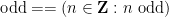
refers to a partially specified integer. Under these conventions, it now becomes theoretically possible that the class one is drawing from becomes empty, and instantiation becomes vacuous. For instance, with our conventions, ${\hbox{odd perfect}}$ refers to a partially specified odd perfect number, which is conjectured to not exist. As it turns out, our notation can handle instances of empty classes without difficulty (basically thanks to the concept of a vacuous truth), but we will avoid dwelling on this edge case much here since this concept is not intuitive for beginners. (But if one does want to confront this possibility, one can use a symbol such as ${\perp}$ to denote an instance of the empty class, i.e., an object that has no specifications whatsoever.

The symbol ${|}$ introduced above can now be extended to be a binary operation on partially specified objects, defined by the formula

$\displaystyle \{ x|y \} == \{x\} \cup \{y\}.$

Thus for instance

$\displaystyle \hbox{odd} | \hbox{even} == \hbox{integer}$

and

$\displaystyle x \pm y == (x+y) | (x-y).$

One can then define other logical operations on partially specified objects if one wishes. For instance, we could define an “and” operator ${\&}$ by defining

$\displaystyle \{ x \& y \} == \{x\} \cap \{y\}.$

Thus for instance

$\displaystyle (5 \pm 3) \& (10 \pm 2) == 8,$

$\displaystyle \hbox{odd} \& \hbox{perfect} == \hbox{odd perfect}$

and

$\displaystyle \hbox{odd} \& \hbox{even} == \perp.$

(Here we are deviating from the syntax of regular expression, but I am not insisting that the entirety of mathematical notation conform to that syntax, and in any event regular expressions do not appear to have a direct analogue of this “and” operation.) We leave it to the reader to propose other logical operations on partially specified objects, though the “or” operator ${|}$ and the “and” operator ${\&}$ will suffice for our purposes.

Any operation on completely specified mathematical objects ${x}$ can be extended to partially specified of mathematical objects ${X}$ by applying that operation to arbitrary instances of the class ${\{X\}}$ , with the convention that if a class appears multiple times in an expression, then we allow each instance of that class to take different values. For instance, if ${x, y}$ are partially specified numbers, we can define ${x+y}$ to be the class of all numbers formed by adding an instance of ${x}$ to an instance of ${y}$ (this is analogous to the operation of Minkowski addition for sets, or interval arithmetic in numerical analysis). For example,

$\displaystyle 5 \pm 3 == 5 + (\pm 3) == 2| 8$

and

$\displaystyle \pm 5 \pm 3 == (\pm 5) + (\pm 3) == -8|-2| 2|8$

(recall that there is no requirement that the signs here align). Note that

$\displaystyle (\pm 3)^2 == 9$

but that

$\displaystyle (\pm 3) \times (\pm 3) == \pm 9.$

So we now see the first sign that some care has to be taken with the law of substitution; we have

$\displaystyle x \times x = x^2$

but we do not have

$\displaystyle (\pm 3) \times (\pm 3) == (\pm 3)^2.$

However, the law of substitution works fine as long as the variable being substituted appears exactly once on both sides of the equation.

One can have an unbounded number of partially specified instances of a class, for instance ${\sum_{i=1}^n \pm 1}$ will be the class of all integers between ${-n}$ and ${+n}$ with the same parity as ${n}$ .

Remark 1 When working with signs ${\pm}$ , one sometimes wishes to keep all signs aligned, with ${\mp}$ denoting the sign opposite to ${\pm}$ , thus for instance with this notation one would have the geometric series formula
$\displaystyle (1 \pm \varepsilon)^{-1} = 1 \mp \varepsilon \pm \varepsilon^2 \mp \varepsilon^3 \dots$
whenever ${|\varepsilon| < 1}$ . However, this notation is difficult to place in the framework used in this blog post without causing additional confusion, and as such we will not discuss it further here. (The syntax of regular expressions does have some tools for encoding this sort of alignment, but in first-order logic we also have the perfectly servicable tool of named variables and quantifiers (or plain old mathematical English) to do so also.)

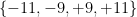
One can also extend binary relations, such as ${<}$ or ${=}$ , to partially specified objects, by requiring that every instance on the left-hand side of the relation relates to some instance on the right-hand side (thus binary relations become ${\Pi_2}$ sentences). Again, if class is instantiated multiple times, we allow different appearances to correspond to different classes. For instance, the statement ${5 \pm 3 \leq 8}$ is true, because every instance of ${5 \pm 3}$ is less than or equal to ${8}$ :

$\displaystyle 5 \pm 3 == (2|8) \leq 8.$

But the statement ${5 \pm 3 \leq 6}$ is false. Similarly, the statement ${8 = 5 \pm 3}$ is true, because ${8}$ is an instance of ${5 \pm 3}$ :

$\displaystyle 8 = (2|8) == 5 \pm 3.$

The statement ${5 \pm 3 < 6 \pm 3}$ is also true, because every instance of ${5 \pm 3}$ is less than some instance of ${6 \pm 3}$ :

$\displaystyle 5 \pm 3 == (2|8) < (3|9) == 6 \pm 3.$

The relationship between a partially specified representative ${x_1|\dots|x_n}$ of a class ${\{x_1|\dots|x_n\}}$ can then be summarised as

$\displaystyle x_1|\dots|x_n \in \{x_1|\dots|x_n\} = \{x_1,\dots,x_n\}.$

Note how this convention treats the left-hand side and right-hand side of a relation involving partially specified expressions asymmetrically. In particular, for partially specified expressions ${x, y}$ , the relation ${x=y}$ is no longer equivalent to ${y=x}$ ; the former states that every instance of ${x}$ is also an instance of ${y}$ , while the latter asserts the converse. For instance, ${3 = \pm 3}$ is a true statement, but ${\pm 3 = 3}$ is a false statement (much as “ ${3}$ is prime” is a true statement (or “ ${3 = \hbox{prime}}$ in our notation), but “primes are ${3}$ ” (or ${\hbox{prime} = 3}$ in our notation) is false). In particular, we see a distinction between equality ${=}$ and equivalence ${==}$ ; indeed, ${x == y}$ holds if and only if ${x=y}$ and ${y=x}$ . On the other hand, as can be easily checked, the following three basic laws of mathematics remain valid for partially specified expressions ${x,y,z}$ :

(i) (Reflexivity) ${x=x}$ .
(ii) (Transitivity) If ${x = y}$ and ${y = z}$ , then ${x=z}$ . Similarly, if ${x < y}$ and ${y < z}$ , then ${x < z}$ , etc..
(iii) (Substitution) If ${x = y}$ , then ${f(x) = f(y)}$ for any function ${f}$ . Similarly, if ${x \leq y}$ , then ${f(x) \leq f(y)}$ for any monotone function ${f}$ , etc..

These conventions for partially specified expressions align well with informal mathematical English. For instance, as discussed in the introduction, the assertion

$\displaystyle \hbox{The sum of two odd numbers is an even number}$

can now be expressed as

$\displaystyle \hbox{odd} + \hbox{odd} = \hbox{even}.$

Similarly, the even Goldbach’s conjecture can now be stated as

$\displaystyle \hbox{even number} \& (\hbox{greater than } 2) = \hbox{prime} + \hbox{prime},$

while the Archimedean property of the reals can be reformulated as the assertion that

$\displaystyle \hbox{real} \leq \hbox{natural number} \times \varepsilon$

for any ${\varepsilon > 0}$ . Note also how the equality symbol ${=}$ for partially specified expressions corresponds well with the multiple meanings of the word “is” in English (consider for instance “two plus two is four”, “four is even”, and “the sum of two odd numbers is even”); the set-theoretic counterpart of this concept would be a sort of amalgam of the ordinary equality relation ${=}$ , the inclusion relation ${\in}$ , and the subset relation ${\subset}$ .

There are however a number of caveats one has to keep in mind, though, when dealing with formulas involving partially specified objects. The first, which has already been mentioned, is a lack of symmetry: ${x=y}$ does not imply ${y=x}$ ; similarly, ${x<y}$ does not imply ${y>x}$ . The second is that negation behaves very strangely, so much so that one should basically avoid using partially specified notation for any sentence that will eventually get negated. For instance, observe that the statements ${3 = \pm 3}$ and ${3 \neq \pm 3}$ are both true, while ${\pm 3 = 3}$ and ${\pm 3 \neq 3}$ are both false. In fact, the negation of such statements as ${x=y}$ or ${x \leq y}$ involving partially specified objects usually cannot be expressed succinctly in partially specified notation, and one must resort to using several quantifiers instead. (In the language of the arithmetic hierarchy, the negation of a ${\Pi_2}$ sentence is a ${\Sigma_2}$ sentence, rather than an another ${\Pi_2}$ sentence.)

Another subtlety, already mentioned earlier, arises from our choice to allow different instantiations of the same class to refer to different instances, namely that the law of universal instantiation does not always work if the symbol being instantiated occurs more than once on the left-hand side. For instance, the identity

$\displaystyle x - x = 0$

is of course true for all real numbers ${x}$ , but if one naively substitutes in the partially specified expression ${\pm 1}$ for ${x}$ one obtains the claim

$\displaystyle \pm 1 - (\pm 1) = 0$

which is a false statement under our conventions (because the two instances of the sign ${\pm 1, \pm 1}$ do not have to match). However, there is no problem with repeated instantiations on the right-hand side, as long as there is at most a single instance on the left-hand side. For instance, starting with the identity

$\displaystyle x = 2x - x$

we can validly instantiate the partially specified expression ${\pm 1}$ for ${x}$ to obtain

$\displaystyle \pm 1 = 2(\pm 1) - (\pm 1).$

A common practice that helps avoid these sorts of issues is to keep the partially specified quantities on the right-hand side of one’s relations, or if one is working with a chain of relations such as ${x \leq y \leq z \leq w}$ , to keep the partially specified quantities away from the left-most side (so that ${y}$ , ${z}$ , and ${w}$ are allowed to be multi-valued, but not ${x}$ ). This doesn’t automatically prevent all issues (for instance, one may still be tempted to “cancel” an expression such as ${\pm 1 - (\pm 1)}$ that might arise partway through a chain of relations), but it can reduce the chance of accidentally making an error.

One can of course translate any formula that involves partially specified objects into a more orthodox first-order logic sentence by inserting the relevant quantifiers in the appropriate places – but note that the variables used in quantifiers are always completely specified, rather than partially specified. For instance, if one expands “ ${x = \pm y}$ ” (for some completely specified quantities ${x,y}$ ) as “there exists ${\epsilon = \pm 1}$ such that ${x = \epsilon y}$ “, the quantity ${\epsilon}$ is completely specified; it is not the partially specified ${\pm 1}$ . (If ${x}$ or ${y}$ were also partially specified, the first-order translation of the expression “ ${x = \pm y}$ ” would be more complicated, as it would need more quantifiers.)

One can combine partially specified notation with set builder notation, for instance the set ${\{ x \in {\bf R}: x = \pm 10 \pm 1 \}}$ is just the four-element set ${\{ -11, -9, +9, +11\}}$ , since these are indeed the four real numbers ${x}$ for which the formula ${x = \pm 10 \pm 1}$ is true. I would however avoid combining particularly heavy uses of set-theoretic notation with partially specified notation, as it may cause confusion.

Our examples above of partially specified objects have been drawn from number systems, but one can use this notation for other classes of objects as well. For instance, within the class of functions ${f: {\bf R} \rightarrow {\bf R}}$ from the reals to themselves, one can make assertions like

$\displaystyle \hbox{increasing} + \hbox{increasing} == \hbox{increasing}$

where ${\hbox{increasing}}$ is the class of monotone increasing functions; similarly we have

$\displaystyle - \hbox{increasing} == \hbox{decreasing}$

$\displaystyle \hbox{increasing} | \hbox{decreasing} == \hbox{monotone}$

$\displaystyle \hbox{positive increasing} \cdot \hbox{negative increasing} = \hbox{negative decreasing}$

$\displaystyle \hbox{bounded} \& \hbox{monotone} = \hbox{converges at infinity}$

$\displaystyle \hbox{analytic} = \hbox{smooth} = \hbox{differentiable} = \hbox{continuous} = \hbox{measurable}$

$\displaystyle \hbox{continuous} / \hbox{continuous nonvanishing} = \hbox{continuous}$

$\displaystyle \hbox{square integrable} \cdot \hbox{square integrable} == \hbox{absolutely integrable}$

$\displaystyle {\mathcal F} \hbox{square integrable} == \hbox{square integrable}$

(with ${{\mathcal F}}$ denoting the Fourier transform) and so forth. Or, in the class of topological spaces, we have for instance

$\displaystyle \hbox{compact} \& \hbox{discrete} == \hbox{finite},$

$\displaystyle \hbox{continuous}(\hbox{compact}) = \hbox{compact},$

and

$\displaystyle \pi_1( \hbox{simply connected} ) = \hbox{trivial group}$

while conversely the classifying space construction gives (among other things)

$\displaystyle \hbox{group} == \pi_1( \hbox{topological space} ).$

Restricting to metric spaces, we have the well known equivalences

$\displaystyle \hbox{compact} == \hbox{sequentially compact} == \hbox{complete} \& \hbox{totally bounded}.$

Note in the last few examples, we are genuinely working with proper classes now, rather than sets. As the above examples hopefully demonstrate, mathematical sentences involving partially specified objects can align very well with the syntax of informal mathematical English, as long as one takes care to distinguish the asymmetric equality relation ${=}$ from the symmetric equivalence relation ${==}$ .

As an example of how such notation might be integrated into an actual mathematical argument, we prove a simple and well known topological result in this notation:

Proposition 2 Let ${f: X \rightarrow Y}$ be a continuous bijection from a compact space ${X}$ to a Hausdorff space ${Y}$ . Then ${f}$ is a homeomorphism.

Proof: We have

$\displaystyle f( \hbox{open subset of }X) = f(X \backslash \hbox{closed subset of } X)$

$\displaystyle = Y \backslash f(\hbox{closed subset of } X)$

(since ${f}$ is a bijection)

$\displaystyle = Y \backslash f(\hbox{compact subset of } X)$

(since ${X}$ is compact)

$\displaystyle = Y \backslash (\hbox{compact subset of } Y)$

(since ${f}$ is continuous)

$\displaystyle = Y \backslash (\hbox{closed subset of } Y)$

(since ${Y}$ is Hausdorff)

$\displaystyle = \hbox{open subset of } Y.$

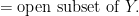Thus ${f}$ is open, hence ${f^{-1}}$ is continuous. Since ${f}$ was already continuous, ${f}$ is a homeomorphism. $\Box$

— 2. Working with parameters —

In order to introduce asymptotic notation, we will need to combine the above conventions for partially specified objects with separate common adjustment to the grammar of mathematical logic, namely the ability to work with ambient parameters. This is a special case of the more general situation of interpreting logic over an elementary topos, but we will not develop the general theory of topoi here. As this adjustment is orthogonal to the adjustments in the preceding section, we shall for simplicity revert back temporarily to the traditional notational conventions for completely specified objects, and not refer to partially specified objects at all in this section.

In the formal language of first-order logic, variables such as ${x,n,X}$ are understood to range in various domains of discourse (e.g., ${x}$ could range in the real numbers, ${n}$ could range in the natural numbers, and ${X}$ in the class of sets). One can then construct various formulas, such as ${P(x,n,X)}$ , in which involve zero or more input variables (known as free variables), and have a truth value in ${\{ \hbox{true}, \hbox{false} \}}$ for any given choice of free variables. For instance, ${P(x,n,X)}$ might be true for some triples ${x \in {\bf R}, n \in {\bf N}, X \in \mathrm{Set}}$ , and false for others. One can create formulas either by applying relations to various terms (e.g., applying the inequality relation ${\leq}$ to the terms ${x+y, z+w}$ gives the formula ${x+y \leq z+w}$ with free variables ${x,y,z,w}$ ), or by combining existing formulas together with logical connectives (such as ${\wedge, \vee, \not, \implies}$ ) or quantifiers ( ${\forall}$ and ${\exists}$ ). Formulas with no free variables (e.g. ${\forall x \forall y: x+y=y+x}$ ) are known as sentences; once one fixes the domains of discourse, sentences are either true or false. We will refer to this first-order logic as orthodox first-order logic, to distinguish it from the parameterised first-order logic we shall shortly introduce.

We now generalise this setup by working relative to some ambient set of parameters – some finite collection of variables that range in some specified sets (or classes) and may be subject to one or more constraints. For instance, one may be working with some natural number parameters ${n,N \in {\bf N}}$ with the constraint ${n \leq N}$ ; we will keep this particular choice of parameters as a running example for the discussion below. Once one selects these parameters, all other variables under consideration are not just single elements of a given domain of discourse, but rather a family of such elements, parameterised by the given parameters; we will refer to these variables as parameterised variables to distinguish them from the orthodox variables of first-order logic. For instance, with the above parameters, when one refers to a real number ${x}$ , one now refers not just to a single element of ${{\bf R}}$ , but rather to a function ${x: (n,N) \mapsto x(n,N)}$ that assigns a real number ${x(n,N)}$ to each choice of parameters ${(n,N)}$ ; we will refer to such a function ${x: (n,N) \mapsto x(n,N)}$ as a parameterised real, and often write ${x = x(n,N)}$ to indicate the dependence on parameters. Each of the ambient parameters can of course be viewed as a parameterised variable, thus for instance ${n}$ can (by abuse of notation) be viewed as the parameterised natural number that maps ${(n,N)}$ to ${n}$ for each choice ${(n,N)}$ of parameters.

The specific ambient set of parameters, and the constraints on them, tends to vary as one progresses through various stages of a mathematical argument, with these changes being announced by various standard phrases in mathematical English. For instance, if at some point a proof contains a sentence such as “Let ${N}$ be a natural number”, then one is implicitly adding ${N}$ to the set of parameters; if one later states “Let ${n}$ be a natural number such that ${n \leq N}$ “, then one is implicitly also adding ${n}$ to the set of parameters and imposing a new constraint ${n \leq N}$ . If one divides into cases, e.g., “Suppose now that ${n}$ is odd… now suppose instead that ${n}$ is even”, then the constraint that ${n}$ is odd is temporarily imposed, then replaced with the complementary constraint that ${n}$ is even, then presumably the two cases are combined and the constraint is removed completely. A bit more subtly, parameters can disappear at the conclusion of a portion of an argument (e.g., at the end of a proof of a lemma or proposition in which the parameter was introduced), replaced instead by a summary statement (e.g., “To summarise, we have shown that whenever ${n,N}$ are natural numbers with ${n \leq N}$ , then …”) or by the statement of the lemma or proposition in whose proof the parameter was temporarily introduced. One can also remove a variable from the set of parameters by specialising it to a specific value.

Any term that is well-defined for individual elements of a domain, is also well-defined for parameterised elements of the domain by pointwise evaluation. For instance, if ${x = x(n,N)}$ and ${y = y(n,N)}$ are parameterised real numbers, one can form the sum ${x+y = (x+y)(n,N)}$ , which is another parameterised real number, by the formula

$\displaystyle (x+y)(n,N) := x(n,N) + y(n,N).$

Given a relation between terms involving parameterised variables, we will interpret the relation as being true (for the given choice of parameterised variables) if it holds for all available choices of parameters ${(n,N)}$ (obeying all ambient constraints), and false otherwise (i.e., if it fails for at least one choice of parameters). For instance, the relation

$\displaystyle x \leq y$

would be interpreted as true if one has ${x(n,N) \leq y(n,N)}$ for all choice of parameters ${(n,N)}$ , and false otherwise.

Remark 3 In the framework of nonstandard analysis, the interpretation of truth is slightly different; the above relation would be considered true if the set of parameters for which the relation holds lies in a given (non-principal) ultrafilter. The main reason for doing this is that it allows for a significantly more general transfer principle than the one available in this setup; however we will not discuss the nonstandard analysis framework further here. (Our setup here is closer in spirit to the “cheap” version of nonstandard analysis discussed in this previous post.)

With this convention an annoying subtlety emerges with regard to boolean connectives (conjunction ${\wedge}$ , disjunction ${\vee}$ , implication ${\implies}$ , and negation ${\neg}$ ), in that one now has to distinguish between internal interpretation of the connectives (applying the connectives pointwise for each choice of parameters before quantifying over parameters), and external interpretation (applying the connectives after quantifying over parameters); there is not a general transfer principle from the former to the latter. For instance, the sentence

$\displaystyle n \hbox{ is odd}$

is false in parameterised logic, since not every choice of parameter ${n}$ is odd. On the other hand, the internal negation

$\displaystyle \neg( n \hbox{ is odd})$

or equivalently

$\displaystyle n \hbox{ is even}$

is also false in parameterised logic, since not every choice of parameter ${n}$ is even. To put it another way, the internal disjunction

$\displaystyle (n \hbox{ is odd}) \vee (n \hbox{ is even})$

is true in parameterised logic, but the individual statements ${n \hbox{ is odd}}$ and ${n \hbox{ is even}}$ are not (so the external disjunction of these statements is false). To maintain this distinction, I will reserve the boolean symbols ( ${\vee, \wedge, \implies, \neg}$ ) for internal boolean connectives, and reserve the corresponding English connectives (“and”, “or”, “implies”, “not”) for external boolean connectives.

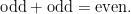
Because of this subtlety, orthodox dichotomies and trichotomies do not automatically transfer over to the parameterised setting. In the orthodox natural numbers, a natural number ${n}$ is either odd or even; but a parameterised natural number ${n}$ could be neither even all the time nor odd all the time. Similarly, given two parameterised real numbers ${x,y}$ , it could be that none of the statements ${x<y}$ , ${x=y}$ , ${x>y}$ are true all the time. However, one can recover these dichotomies or trichotomies by subdividing the parameter space into cases. For instance, in the latter example, one could divide the parameter space into three regions, one where ${x<y}$ is always true, one where ${x=y}$ is always true, and one where ${x>y}$ is always true. If one can prove a single statement in all three subregions of parameter space, then of course this implies the statement in the original parameter space. So in practice one can still use dichotomies and trichotomies in parameterised logic, so long as one is willing to subdivide the parameter space into cases at various stages of the argument and recombine them later.

There is a similar distinction between internal quantification (quantifying over orthodox variables before quantifying over parameters), and external quantification (quantifying over parameterised variables after quantifying over parameters); we will again maintain this distinction by reserving the symbols ${\forall, \exists}$ for internal quantification and the English phrases “for all” and “there exists” for external quantification. For instance, the assertion

$\displaystyle x+y = y+x \hbox{ for all } x, y \in {\bf R}$

when interpreted in parameterised logic, means that for all parameterised reals ${x: (n,N) \mapsto x(n,N)}$ and ${y: (n,N) \mapsto y(n,N)}$ , the assertion ${x(n,N)+ y(n,N) = y(n,N) + x(n,N)}$ holds for all ${n,N}$ . In this case it is clear that this assertion is true and is in fact equivalent to the orthodox sentence ${\forall x,y \in {\bf R}: x+y = y+x}$ . More generally, we do have a restricted transfer principle in that any true sentence in orthodox logic that involves only quantifiers and no boolean connectives, will transfer over to parameterised logic (at least if one is willing to use the axiom of choice freely, which we will do in this post). We illustrate this (somewhat arbitrarily) with the Lagrange four square theorem

$\displaystyle \forall m \in {\bf N} \exists a,b,c,d \in {\bf N}: m = a^2+b^2+c^2+d^2. \ \ \ \ \ (5)$

This sentence, true in orthodox logic, implies the parameterised assertion that for every parameterised natural number ${m: (n,N) \mapsto m(n,N)}$ , there exist parameterised natural numbers ${a: (n,N) \mapsto a(n,N)}$ , ${b: (n,N) \mapsto b(n,N)}$ , ${c: (n,N) \mapsto c(n,N)}$ , ${d: (n,N) \mapsto d(n,N)}$ , such that ${m(n,N) = a(n,N)^2 + b(n,N)^2 + c(n,N)^2 + d(n,N)^2}$ for all choice of parameters ${(n,N)}$ . To see this, we can Skolemise the four-square theorem (5) to obtain functions ${\tilde a: m \mapsto \tilde a(m)}$ , ${\tilde b: m \mapsto \tilde b(m)}$ , ${\tilde c: m \mapsto \tilde c(m)}$ , ${\tilde d: m \mapsto \tilde d(m)}$ such that

$\displaystyle m = \tilde a(m)^2 + \tilde b(m)^2 + \tilde c(m)^2 + \tilde d(m)^2$

for all orthodox natural numbers ${m}$ . Then to obtain the parameterised claim, one simply sets ${a(n,N) := \tilde a(m(n,N))}$ , ${b(n,N) := \tilde b(m(n,N))}$ , ${c(n,N) := \tilde c(m(n,N))}$ , and ${d(n,N) := \tilde d(m(n,N))}$ . Similarly for other sentences that avoid boolean connectives. (There are some further classes of sentences that use boolean connectives in a restricted fashion that can also be transferred, but we will not attempt to give a complete classification of such classes here; in general it is better to work out some examples of transfer by hand to see what can be safely transferred and which ones cannot.)

So far this setup is not significantly increasing the expressiveness of one’s language, because any statement constructed so far in parameterised logic can be quickly translated to an equivalent (and only slightly longer) statement in orthodox logic. However, one gains more expressive power when one allows one or more of the parameterised variables to have a specified type of dependence on the parameters, and in particular depending only on a subset of the parameters. For instance, one could introduce a real number ${C}$ which is an absolute constant in the sense that it does not depend on either of the parameters ${n,N}$ ; these are a special type of parameterised real, in much the same way that constant functions are a special type of function. Or one could consider a parameterised real ${a = a(N)}$ that depends on ${N}$ but not on ${n}$ , or a parameterised real ${b = b(n)}$ that depends on ${n}$ but not on ${N}$ . (One could also place other types of constraints on parameterised quantities, such as continuous or measurable dependence on the parameters, but we will not consider these variants here.)

By quantifying over these restricted classes of parameterised functions, one can now efficiently write down a variety of statements in parameterised logic, of types that actually occur quite frequently in analysis. For instance, we can define a parameterised real ${x = x(n,N)}$ to be bounded if there exists an absolute constant ${C}$ such that ${|x| \leq C}$ ; one can of course write this assertion equivalently in orthodox logic as

$\displaystyle \exists C \forall n,N: ((n \leq N) \implies (|x(n,N)| \leq C).$

One can also define the stronger notion of ${x}$ being ${1}$ -bounded, by which we mean ${|x| \leq 1}$ , or in orthodox logic

$\displaystyle \forall n,N: ((n \leq N) \implies (|x(n,N)| \leq 1).$

In the opposite direction, we can assert the weaker statement that ${x = x(n,N)}$ is bounded in magnitude by a quantity ${C = C(N)}$ that depends on ${N}$ but not on ${n}$ ; in orthodox logic this becomes

$\displaystyle \forall N \exists C \forall n \leq N: |x(n,N)| \leq C.$

As before, each of the example statements in parameterised logic can be easily translated into a statement in traditional logic. On the other hand, consider the assertion that a parameterised real ${x = x(n,N)}$ is expressible as the sum ${x = y + z}$ of a quantity ${y = y(n)}$ depending only on ${n}$ and a quantity ${z = z(N)}$ depending on ${N}$ . (For instance, the parameterised real ${x = (N+n)(N-n) = N^2 - n^2}$ would be of this form, but the parameterised real ${x = Nn}$ cannot.) Now it becomes significantly harder to translate this statement into first-order logic! One can still do so fairly readily using second-order logic (in which one also is permitted to quantify over operators as well as variables), or by using the language of set theory (so that one can quantify over a set of functions of various forms). Indeed if one is parameterising over proper classes rather than sets, it is even possible to create sentences in parameterised logic that are non-firstorderisable; see this previous blog post for more discussion.

Another subtle distinction that arises once one has parameters is the distinction between “internal” or `parameterised” sets (sets depending on the choice of parameters), and external sets (sets of parameterised objects). For instance, the interval ${[n,N]}$ is an internal set – it assigns an orthodox set ${\{ x \in {\bf R}: n \leq x \leq N \}}$ of reals to each choice of parameters ${(n,N)}$ ; elements of this set consist of all the parameterised reals ${x = x(n,N)}$ such that ${n \leq x(n,N) \leq N}$ for all ${n,N}$ . On the other hand, the collection ${{\mathcal O}(1)}$ of bounded reals – i.e., parameterised reals ${x = x(n,N)}$ such that there is a constant ${C}$ for which ${|x(n,N)| \leq C}$ for all choices of parameters ${(n,N)}$ – is not an internal set; it does not arise from taking an orthodox set of reals ${X(n,N)}$ for each choice of parameters. (Indeed, if it did do so, since every constant real is bounded, each ${X(n,N)}$ would contain all of ${{\bf R}}$ , which would make ${{\mathcal O}(1)}$ the set of all parameterised reals, rather than just the bounded reals.) To maintain this distinction, we will reserve set builder notation such as ${\{ x \in X: P(x) \}}$ for internally defined sets, and use English words (such as “the collection of all bounded parameterised reals”) to denote external sets. In particular, we do not make sense of such expressions as ${\{ x \in {\bf R}: x \hbox{ bounded} \}}$ (or ${\{ x \in {\bf R}: x = O(1) \}}$ , once asymptotic notation is introduced). In general, I would recommend that one avoids combining asymptotic notation with heavy use of set theoretic notation, unless one knows exactly what one is doing.

— 3. Asymptotic notation —

We now simultaneously introduce the two extensions to orthodox first order logic discussed in previous sections. In other words,

We permit the use of partially specified mathematical objects in one’s mathematical statements (and in particular, on either side of an equation or inequality).
We allow all quantities to depend on one or more of the ambient parameters.

In particular, we allow for the use of partially specified mathematical quantities that also depend on one or more of the ambient parameters. This allows us now formally introduce asymptotic notation. There are many variants of this notation, but here is one set of asymptotic conventions that I for one like to use:

Definition 4 (Asymptotic notation) Let ${X}$ be a non-negative quantity (possibly depending on one or more of the ambient parameters).

We use ${O(X)}$ to denote a partially specified quantity in the class of quantities ${Y}$ (that can depend on one or more of the ambient parameters) that obeys the bound ${|Y| \leq CX}$ for some absolute constant ${C > 0}$ . More generally, given some ambient parameters ${\lambda_1,\dots,\lambda_k}$ , we use ${O_{\lambda_1,\dots,\lambda_k}(X)}$ to denote a partially specified quantity in the class of quantities ${Y}$ that obeys the bound ${|Y| \leq C_{\lambda_1,\dots,\lambda_k}(X)}$ for some constant ${C > 0}$ that can depend on the ${\lambda_1,\dots,\lambda_k}$ parameters, but not on the other ambient parameters.

We also use ${X \ll Y}$ or ${Y \gg X}$ as a synonym for ${X = O(Y)}$ , and ${X \asymp Y}$ as a synonym for ${X \ll Y \ll X}$ . (In some fields of analysis, ${X \lesssim Y}$ , ${X \gtrsim Y}$ , and ${X \sim Y}$ are used instead of ${X \ll Y}$ , ${X \gg Y}$ , and ${X \asymp Y}$ .)

If ${x}$ is a parameter and ${x_*}$ is a limiting value of that parameter (i.e., the parameter space for ${x}$ and ${x_*}$ both lie in some topological space, with ${x_*}$ an adherent point of that parameter space), we use ${o_{x \rightarrow \infty}(X)}$ to denote a partially specified quantity in the class of quantities ${Y}$ (that can depend on ${x}$ as well as the other the ambient parameters) that obeys a bound of the form ${|Y| \leq c(x) X}$ for some quantity ${c(x) > 0}$ depending only on ${x}$ such that ${c(x) \rightarrow 0}$ 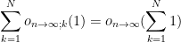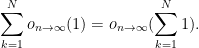as ${x \rightarrow x_*}$ . More generally, given some further ambient parameters ${\lambda_1,\dots,\lambda_k}$ , we use ${o_{x \rightarrow x_*; \lambda_1,\dots,\lambda_k}(X)}$ to denote a partially specified quantity in the class of quantities ${Y}$ that obey a bound of the form ${|Y| \leq c_{\lambda_1,\dots,\lambda_k}(x) X}$ , where ${c_{\lambda_1,\dots,\lambda_k}(x) > 0}$ depends on ${\lambda_1,\dots,\lambda_k,x}$ and goes to zero as ${x \rightarrow x_*}$ .

Sometimes (by explicitly declaring one will do so) one suppresses the dependence on one or more of the additional parameters ${\lambda_1,\dots,\lambda_k}$ , and/or the asymptotic limit ${x \rightarrow x_*}$ , in order to reduce clutter.

Thus, for instance, ${n}$ is a free variable taking values in the natural numbers, and ${f(n), g(n), h(n)}$ are quantities depending on ${n}$ , then the statement ${f(n) = g(n) + O(h(n))}$ denotes the assertion that ${f(n) = g(n) + k(n)}$ for all natural numbers ${n}$ , where ${k(n)}$ is another quantity depending on ${n}$ such that ${|k(n)| \leq C h(n)}$ for all ${n}$ , and some absolute constant ${C}$ independent of ${n}$ . Similarly, ${f(n) \leq g(n) + O(h(n))}$ denotes the assertion that ${f(n) \leq g(n) + k(n)}$ for all natural numbers ${n}$ , where ${k(n)}$ is as above.

For a slightly more sophisticated example, consider the statement

$\displaystyle O(n) + O(n^2) \leq O(n^2), \ \ \ \ \ (6)$

where again ${n}$ is a free variable taking values in the natural numbers. Using the conventions for multi-valued expressions, we can translate this expression into first-order logic as the assertion that whenever ${f(n), g(n)}$ are quantities depending on ${n}$ such that there exists a constant ${C_1}$ such that ${|f(n)| \leq C_1 n}$ for all natural numbers ${n}$ , and there exists a constant ${C_2}$ such that ${|g(n)| \leq C_2 n^2}$ for all natural numbers ${n}$ , then we have ${f(n)+g(n) \leq h(n)}$ for all ${n}$ , where ${h}$ is a quantity depending on natural numbers ${n}$ with the property that there exists a constant ${C_3}$ such that ${|h(n)| \leq C_3 n^2}$ . Note that the first-order translation of (6) is substantially longer than (6) itself; and once one gains familiarity with the big-O notation, (6) can be deciphered much more quickly than its formal first-order translation.

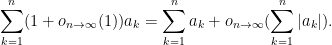
It can be instructive to rewrite some basic notions in analysis in this sort of notation, just to get a slightly different perspective. For instance, if ${f: {\bf R} \rightarrow {\bf R}}$ is a function, then:

${f}$ is continuous iff one has ${f(y) = f(x) + o_{y \rightarrow x; f,x}(1)}$ for all ${x,y \in {\bf R}}$ .
${f}$ is uniformly continuous iff one has ${f(y) = f(x) + o_{|y-x| \rightarrow 0; f}(1)}$ for all ${x,y \in {\bf R}}$ .
A sequence ${F = (f_n)_{n \in {\bf N}}}$ of functions is equicontinuous if one has ${f_n(y) = f_n(x) + o_{y \rightarrow x; F,x}(1)}$ for all ${x,y \in {\bf R}}$ and ${n \in {\bf N}}$ (note that the implied constant depends on the family ${F}$ , but not on the specific function ${f_n}$ or on the index ${n}$ ).
A sequence ${F = (f_n)_{n \in {\bf N}}}$ of functions is uniformly equicontinuous if one has ${f_n(y) = f_n(x) + o_{|y-x| \rightarrow 0; F}(1)}$ for all ${x,y \in {\bf R}}$ and ${n \in {\bf N}}$ .
${f}$ is differentiable iff one has ${f(y) = f(x) + (y-x) f'(x) + o_{y \rightarrow x; f,x}(|y-x|)}$ for all ${x,y \in {\bf R}}$ .
Similarly for uniformly differentiable, equidifferentiable, etc..

Remark 5 One can define additional variants of asymptotic notation such as ${\Omega(X)}$ , ${\omega(X)}$ , or ${\Theta(X)}$ ; see this wikipedia page for some examples. See also the related notion of “sufficiently large” or “sufficiently small”. However, one can usually reformulate such notations in terms of the above-mentioned asymptotic notations with a little bit of rearranging. For instance, the assertion
$\displaystyle \hbox{For all sufficiently large } n, P(n) \hbox{ is true}$
can be rephrased as an alternative:
$\displaystyle \hbox{If } n \hbox{ is a natural number, then } P(n) \hbox{, or } n = O(1).$

When used correctly, asymptotic notation can suppress a lot of distracting quantifiers (“there exists a ${C}$ such that for every ${n}$ one has…”) or temporary notation which is introduced once and then discarded (“where ${C}$ is a constant, not necessarily the same as the constant ${C}$ from the preceding line…”). It is particularly well adapted to situations in which the order of magnitude of a quantity of interest is of more importance than its exact value, and can help capture precisely such intuitive notions as “large”, “small”, “lower order”, “main term”, “error term”, etc.. Furthermore, I find that analytic assertions phrased using asymptotic notation tend to align better with the natural sentence structure of mathematical English than their logical equivalents in other notational conventions (e.g. first-order logic).

On the other hand, the notation can be somewhat confusing to use at first, as expressions involving asymptotic notation do not always obey the familiar laws of mathematical deduction if applied blindly; but the failures can be explained by the changes to orthodox first order logic indicated above. For instance, if ${n}$ is a positive integer (which we will assume to be at least say ${100}$ , in order to make sense of quantities such as ${\log\log n}$ ), then

(i) (Asymmetry of equality) We have ${O(n) = O(n^2)}$ , but it is not true that ${O(n^2) = O(n)}$ . In the same spirit, ${O(n) \leq O(n^2)}$ is a true statement, but ${O(n^2) \geq O(n)}$ is a false statement. Similarly for the ${o()}$ notation. This of course stems from the asymmetry of the equality relation ${=}$ that arises once one introduces partially specified objects.
(ii) (Intransitivity of equality) We have ${n+1 = O(n)}$ , and ${n+2 = O(n)}$ , but ${n+1 \neq n+2}$ . This is again stemming from the asymmetry of the equality relation.
(iii) (Incompatibility with functional notation) ${O(n)}$ generally refers to a function of ${n}$ , but ${O(1)}$ usually does not refer to a function of ${1}$ (for instance, it is true that ${\frac{1}{n} = O(1)}$ ). This is a slightly unfortunate consequence of the overloaded nature of the parentheses symbols in mathematics, but as long as one keeps in mind that ${O}$ and ${o}$ are not function symbols, one can avoid ambiguity.
(iv) (Incompatibility with mathematical induction) We have ${O(n+1)=O(n)}$ , and more generally ${O(n+k+1)=O(n+k)}$ for any ${k \geq 1}$ , but one cannot blindly apply induction and conclude that ${O(n+k)=O(n)}$ for all ${n,k \geq 1}$ (with ${k}$ viewed as an additional parameter). This is because to induct on an internal parameter such as ${n}$ , one is only allowed to use internal predicates ${P(n)}$ ; the assertion ${O(n+1)=O(n)}$ , which also quantifies externally over some implicit constants ${C}$ , is not an internal predicate. However, external induction is still valid, permitting one to conclude that ${O(n+k)=O(n)}$ for any fixed (external) ${k \geq 1}$ , or equivalently that ${O(n+k) = O_k(n)}$ if ${k}$ is now viewed instead as a parameter.
(v) (Failure of the law of generalisation) Every specific (or “fixed”) positive integer, such as ${57}$ , is of the form ${O(1)}$ , but the positive integer ${n}$ is not of the form ${O(1)}$ . (Again, this can be fixed by allowing implied constants to depend on the parameter one is generalising over.) Like (iv), this arises from the need to distinguish between external (fixed) variables and internal parameters.
(vi) (Failure of the axiom schema of specification) Given a set ${X}$ and a predicate ${P(x)}$ involving elements ${x}$ of ${X}$ , the axiom of specification allows one to use set builder notation to form the set ${\{ x \in X: P(x) \}}$ . However, this is no longer possible if ${P}$ involves asymptotic notation. For instance, one cannot form the “set” ${\{ x \in {\bf R}: x = O(1) \}}$ of bounded real numbers, which somehow manages to contain all fixed numbers such as ${57}$ , but not any unbounded free parameters such as ${n}$ . (But, if one uses the nonstandard analysis formalism, it becomes possible again to form such sets, with the important caveat that such sets are now external sets rather than internal sets. For instance, the external set ${\{ x \in {}^* {\bf R}: x = O(1) \}}$ of bounded nonstandard reals becomes a proper subring of the ring of nonstandard reals.) This failure is again related to the distinction between internal and external predicates.
(vii) (Failure of trichotomy) For non-asymptotic real numbers ${X,Y}$ , exactly one of the statements ${X<Y}$ , ${X=Y}$ , ${X>Y}$ hold. As discussed in the previous section, this is not the case for asymptotic quantities: none of the three statements ${O(|\sin(n)|) = O(|\cos(n)|)}$ , ${O(|\sin(n)|) > O(|\cos(n)|)}$ , or ${O(|\sin(n)|) < O(|\cos(n)|)}$ are true, while all three of the statements ${O(n) < O(n)}$ , ${O(n) = O(n)}$ , and ${O(n) > O(n)}$ are true. (This trichotomy can however be restored by using the nonstandard analysis formalism, or (in some cases) by restricting ${n}$ to an appropriate subsequence whenever necessary.)
(viii) (Unintuitive interaction with ${\neq}$ ) Asymptotic notation interacts in strange ways with the ${\neq}$ symbol, to the extent that combining the two together is not recommended. For instance, the statement ${O(n) \neq O(n)}$ is a true statement, because for any expression ${a_n}$ of order ${a_n = O(n)}$ , one can find another expression ${b_n}$ of order ${b_n = O(n)}$ such that ${a_n \neq b_n}$ for all ${n}$ . Instead of using statements such as ${X \neq Y}$ in which one of ${X,Y}$ contain asymptotic notation, I would instead recommend using the different statement “it is not the case that ${X=Y}$ “, e.g. “it is not the case that ${O(n^2)=O(n)}$ “. And even then, I would generally only use negation of asymptotic statements in order to demonstrate the incorrectness of some particular argument involving asymptotic notation, and not as part of any positive argument involving such notations. These issues are of course related to (vii).
(ix) (Failure of cancellation law) We have ${O(n) + O(n) = O(n)}$ , but one cannot cancel one of the ${O(n)}$ terms and conclude that ${O(n) = 0}$ . Indeed, ${O(n)-O(n)}$ is not equal to ${0}$ in general. (For instance, ${2n = O(n)}$ and ${n=O(n)}$ , but ${2n-n \neq 0}$ .) More generally, ${O(X)-O(Y)}$ is not in general equal to ${O(X-Y)}$ or even to ${O(|X-Y|)}$ (although there is an important exception when one of ${X,Y}$ dominates the other). Similarly for the ${o()}$ notation. This stems from the care one has to take in the law of substitution when working with partially specified quantities that appear multiple times on the left-hand side.
(x) ( ${O()}$ , ${o()}$ do not commute with signed multiplication) If ${X,Y}$ are non-negative, then ${X \cdot O(Y) = O(XY)}$ and ${X \cdot o_{n \rightarrow \infty}(Y) = o_{n \rightarrow \infty}(XY)}$ . However, these laws do not work if ${X}$ is signed; indeed, as currently defined ${O(XY)}$ and ${o_{n \rightarrow \infty}(XY)}$ do not even make sense. Thus for instance ${-O(n)}$ cannot be written as ${O(-n)}$ . (However, one does have ${X \cdot O(Y) = O(|X| Y)}$ and ${X \cdot o_{n \rightarrow \infty}(Y) = o_{n \rightarrow \infty}(|X| Y)}$ when ${X}$ is signed.) This comes from the absolute values present in the ${O()}$ -notation. For beginners, I would recommend not placing any signed quantities inside the ${O()}$ and ${o()}$ symbols if at all possible.
(xi) ( ${O()}$ need not distribute over summation) For each fixed ${k}$ , ${k = O(1)}$ , and ${\sum_{k=1}^n 1 = n}$ , but it is not the case that ${\sum_{k=1}^n k = O(n)}$ . This example seems to indicate that the assertion ${\sum_{k=1}^n O(1) = O( \sum_{k=1}^n 1 )}$ is not true, but that is because we have conflated an external (fixed) quantity ${k}$ with an internal parameter ${k}$ (the latter being needed to define the summation ${\sum_{k=1}^n}$ ). The more precise statements (with ${k}$ now consistently an internal parameter) are that ${k = O_k(1)}$ , and that the assertion ${\sum_{k=1}^n O_k(1) = O( \sum_{k=1}^n 1 )}$ is not true, but the assertion ${\sum_{k=1}^n O(1) = O( \sum_{k=1}^n 1 )}$ is still true (why?).
(xii) ( ${o()}$ does not distribute over summation, I) Let ${\varepsilon_k(n) := \exp(\exp(n)) 1_{k \geq \log\log n - 1}}$ , then for each fixed ${k}$ one has ${\varepsilon_k(n) = o_{n \rightarrow \infty}(1)}$ ; however, ${\sum_{k=1}^{\log\log n} \varepsilon_k(n) \geq \exp(\exp(n))}$ . Thus an expression of the form ${\sum_{k=1}^{\log\log n} o_{n \rightarrow \infty}(1)}$ can in fact grow extremely fast in ${n}$ (and in particular is not of the form ${o_{n \rightarrow \infty}(\log\log n)}$ or even ${O(\log\log n)}$ ). Of course, one could replace ${\log\log n}$ here by any other growing function of ${n}$ . This is a similar issue to (xi); it shows that the assertion
$\displaystyle \sum_{k=1}^N o_{n \rightarrow \infty;k}(1) = o_{n \rightarrow \infty}(\sum_{k=1}^N 1)$
can fail, but if one has uniformity in the ${k}$ parameter then things are fine:
$\displaystyle \sum_{k=1}^N o_{n \rightarrow \infty}(1) = o_{n \rightarrow \infty}(\sum_{k=1}^N 1).$
(xiii) ( ${o()}$ does not distribute over summation, II) In the previous example, the ${o_{n \rightarrow \infty}(1)}$ summands were not uniformly bounded. If one imposes uniform boundedness, then one now recovers the ${O()}$ bound, but one can still lose the ${o()}$ bound. For instance, let ${\varepsilon_k(n) := 1_{k \geq \log\log n}}$ , then ${\varepsilon_k(n)}$ is now uniformly bounded in magnitude by ${1}$ , and for each fixed ${k}$ one has ${\varepsilon_k(n) = o_{n \rightarrow \infty}(1)}$ ; however, ${\sum_{k=1}^n \varepsilon_k(n) = n - O(\log\log n)}$ . Thus, viewing ${k}$ now as a parameter, the expression ${\sum_{k=1}^n o_{n \rightarrow \infty;k}(1)}$ is bounded by ${O(n)}$ , but not by ${o_{n \rightarrow \infty}(n)}$ . (However, one can write ${\sum_{k=1}^n o_{n \rightarrow \infty}(a_k) = o_{n \rightarrow \infty}(\sum_{k=1}^n |a_k|)}$ since by our conventions the implied decay rates in the ${o_{n \rightarrow \infty}(a_k)}$ summands are uniform in ${n}$ .)
(xiv) ( ${o()}$ does not distribute over summation, III) If ${a_k}$ are non-negative quantities, and one has a summation of the form ${\sum_{k=1}^n (1+o_{n \rightarrow \infty}(1)) a_k}$ (noting here that the decay rate is not allowed to depend on ${k}$ ), then one can “factor out” the ${1+o_{n \rightarrow \infty}(1)}$ term to write this summation as ${(1 + o_{n \rightarrow \infty}(1)) (\sum_{k=1}^n a_k)}$ . However this is far from being true if the sum ${\sum_{k=1}^n a_k}$ exhibits significant cancellation. This is most vivid in the case when the sum ${\sum_{k=1}^n a_k}$ actually vanishes. For another example, the sum ${\sum_{k=1}^{n} (1 + \frac{(-1)^k}{\log\log n}) (-1)^k}$ is equal to ${\frac{n}{\log\log n} + O(1)}$ , despite the fact that ${1 + \frac{(-1)^k}{\log\log n} = 1 + o_{n \rightarrow\infty}(1)}$ uniformly in ${k}$ , and that ${\sum_{k=1}^n (-1)^k = O(1)}$ . For oscillating ${a_k}$ , the best one can say in general is that
$\displaystyle \sum_{k=1}^n (1+o_{n \rightarrow \infty}(1)) a_k = \sum_{k=1}^n a_k + o_{n \rightarrow \infty}( \sum_{k=1}^n |a_k| ).$
Similarly for the ${O()}$ notation. I see this type of error often among beginner users of asymptotic notation. Again, the general remedy is to avoid putting any signed quantities inside the ${O()}$ or ${o()}$ notations.

Perhaps the quickest way to develop some basic safeguards is to be aware of certain “red flags” that indicate incorrect, or at least dubious, uses of asymptotic notation, as well as complementary “safety indicators” that give more reassurance that the usage of asymptotic notation is valid. From the above examples, we can construct a small table of such red flags and safety indicators for any expression or argument involving asymptotic notation:

Red flag Safety indicator Signed quantities in RHS Absolute values in RHS Casually using iteration/induction Explicitly allowing bounds to depend on length of iteration/induction Casually summing an unbounded number of terms Keeping number of terms bounded and/or ensuring uniform bounds on each term Casually changing a “fixed” quantity to a “variable” or “bound” one Keeping track of what parameters implied constants depend on Casually establishing lower bounds or asymptotics Establishing upper bounds and/or being careful with signs and absolute values Signed algebraic manipulations (e.g., cancellation law) Unsigned algebraic manipulations ${X \neq Y}$ Negation of ${X=Y}$ ; or, better still, avoiding negation altogether Swapping LHS and RHS Not swapping LHS and RHS Using trichotomy of order Not using trichotomy of order Set-builder notation Not using set-builder notation (or, in non-standard analysis, distinguishing internal sets from external sets)

When I say here that some mathematical step is performed “casually”, I mean that it is done without any of the additional care that is necessary when this step involves asymptotic notation (that is to say, the step is performed by blindly applying some mathematical law that may be valid for manipulation of non-asymptotic quantities, but can be dangerous when applied to asymptotic ones). It should also be noted that many of these red flags can be disregarded if the portion of the argument containing the red flag is free of asymptotic notation. For instance, one could have an argument that uses asymptotic notation in most places, except at one stage where mathematical induction is used, at which point the argument switches to more traditional notation (using explicit constants rather than implied ones, etc.). This is in fact the opposite of a red flag, as it shows that the author is aware of the potential dangers of combining induction and asymptotic notation. Similarly for the other red flags listed above; for instance, the use of set-builder notation that conspicuously avoids using the asymptotic notation that appears elsewhere in an argument is reassuring rather than suspicious.

If one finds oneself trying to use asymptotic notation in a way that raises one or more of these red flags, I would strongly recommend working out that step as carefully as possible, ideally by writing out both the hypotheses and conclusions of that step in non-asymptotic language (with all quantifiers present and in the correct order), and seeing if one can actually derive the conclusion from the hypothesis by traditional means (i.e., without explicit use of asymptotic notation ). Conversely, if one is reading a paper that uses asymptotic notation in a manner that casually raises several red flags without any apparent attempt to counteract them, one should be particularly skeptical of these portions of the paper.

As a simple example of asymptotic notation in action, we give a proof that convergent sequences also converge in the Césaro sense:

Proposition 6 If ${\vec x = (x_n)_{n \in {\bf N}}}$ is a sequence of real numbers converging to a limit ${L}$ , then the averages ${\frac{1}{N} \sum_{n=1}^N x_n}$ also converge to ${L}$ as ${N \rightarrow \infty}$ .

Proof: Since ${x_n}$ converges to ${L}$ , we have

$\displaystyle x_n = L + o_{n \rightarrow \infty; \vec x}(1)$

so in particular for any ${M \geq 1}$ we have

$\displaystyle x_n = L + o_{M \rightarrow \infty; \vec x}(1)$

whenever ${n > M}$ . For ${N \geq M}$ , we thus have

$\displaystyle \frac{1}{N} \sum_{n=1}^N x_n = \frac{1}{N} ( \sum_{n=1}^M x_n + \sum_{n=M+1}^N x_n)$

$\displaystyle = \frac{1}{N}( O_{M,\vec x}(1) + \sum_{n=M+1}^N (L + o_{M \rightarrow \infty; \vec x}(1)))$

$\displaystyle = \frac{1}{N}( O_{M,\vec x}(1) + (N-M) L + o_{M \rightarrow \infty; \vec x}(N))$

$\displaystyle = O_{M,\vec x}(1/N) + L - O_{M,L}(1/N) + o_{M \rightarrow \infty; \vec x}(1)$

$\displaystyle = L + o_{M \rightarrow \infty; \vec x}(1) + o_{N \rightarrow \infty; \vec x, M, L}(1)$

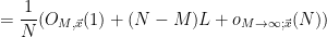
whenever ${N \geq M}$ . Setting ${M}$ to grow sufficiently slowly to infinity as ${N \rightarrow \infty}$ (for fixed ${\vec x, \vec L}$ ), we may simplify this to

$\displaystyle \frac{1}{N} \sum_{n=1}^N x_n = o_{N \rightarrow \infty; \vec x, L}(1)$

for all ${N \geq 1}$ , and the claim follows. $\Box$