Bounding sums or integrals of non-negative quantities

What's new 2023-10-01

A common task in analysis is to obtain bounds on sums

$\displaystyle \sum_{n \in A} f(n)$

or integrals

$\displaystyle \int_A f(x)\ dx$

where ${A}$ is some simple region (such as an interval) in one or more dimensions, and ${f}$ is an explicit (and elementary) non-negative expression involving one or more variables (such as ${n}$ or ${x}$ , and possibly also some additional parameters. Often, one would be content with an order of magnitude upper bound such as

$\displaystyle \sum_{n \in A} f(n) \ll X$

$\displaystyle \int_A f(x)\ dx \ll X$

where we use ${X \ll Y}$ (or ${Y \gg X}$ or ${X = O(Y)}$ ) to denote the bound ${|X| \leq CY}$ for some constant ${C}$ ; sometimes one wishes to also obtain the matching lower bound, thus obtaining

$\displaystyle \sum_{n \in A} f(n) \asymp X$

$\displaystyle \int_A f(x)\ dx \asymp X$

where ${X \asymp Y}$ is synonymous with ${X \ll Y \ll X}$ . Finally, one may wish to obtain a more precise bound, such as

$\displaystyle \sum_{n \in A} f(n) = (1+o(1)) X$

where ${o(1)}$ is a quantity that goes to zero as the parameters of the problem go to infinity (or some other limit). (For a deeper dive into asymptotic notation in general, see this previous blog post.)

Here are some typical examples of such estimation problems, drawn from recent questions on MathOverflow:

(i) (From this question) If ${d,p \geq 1}$ and ${a>d/p}$ , is the expression
$\displaystyle \sum_{j \in {\bf Z}} 2^{(\frac{d}{p}+1-a)j} \int_0^\infty e^{-2^j s} \frac{s^a}{1+s^{2a}}\ ds$
finite?
(ii) (From this question) If ${h,m \geq 1}$ , how can one show that
$\displaystyle \sum_{d=0}^\infty \frac{2d+1}{2h^2 (1 + \frac{d(d+1)}{h^2}) (1 + \frac{d(d+1)}{h^2m^2})^2} \ll 1 + \log(m^2)?$
(iii) (From this question) Can one show that
$\displaystyle \sum_{k=1}^{n-1} \frac{k^{2n-4k-3}(n^2-2nk+2k^2)}{(n-k)^{2n-4k-1}} = (c+o(1)) \sqrt{n}$
as ${n \rightarrow \infty}$ for an explicit constant ${c}$ , and what is this constant?

Compared to other estimation tasks, such as that of controlling oscillatory integrals, exponential sums, singular integrals, or expressions involving one or more unknown functions (that are only known to lie in some function spaces, such as an ${L^p}$ space), high-dimensional geometry (or alternatively, large numbers of random variables), or number-theoretic structures (such as the primes), estimation of sums or integrals of non-negative elementary expressions is a relatively straightforward task, and can be accomplished by a variety of methods. The art of obtaining such estimates is typically not explicitly taught in textbooks, other than through some examples and exercises; it is typically picked up by analysts (or those working in adjacent areas, such as PDE, combinatorics, or theoretical computer science) as graduate students, while they work through their thesis or their first few papers in the subject.

Somewhat in the spirit of this previous post on analysis problem solving strategies, I am going to try here to collect some general principles and techniques that I have found useful for these sorts of problems. As with the previous post, I hope this will be something of a living document, and encourage others to add their own tips or suggestions in the comments.

— 1. Asymptotic arithmetic —

Asymptotic notation is designed so that many of the usual rules of algebra and inequality manipulation continue to hold, with the caveat that one has to be careful if subtraction or division is involved. For instance, if one knows that ${A \ll X}$ and ${B \ll Y}$ , then one can immediately conclude that ${A + B \ll X+Y}$ and ${AB \ll XY}$ , even if ${A,B}$ are negative (note that the notation ${A \ll X}$ or ${B \ll Y}$ automatically forces ${X,Y}$ to be non-negative). Equivalently, we have the rules

$\displaystyle O(X) + O(Y) = O(X+Y); \quad O(X) \cdot O(Y) = O(XY)$

and more generally we have the triangle inequality

$\displaystyle \sum_\alpha O(X_\alpha) = O( \sum_\alpha X_\alpha ).$

(Again, we stress that this sort of rule implicitly requires the ${X_\alpha}$ to be non-negative. As a rule of thumb, if your calculations have arrived at a situation where a signed or oscillating sum or integral appears inside the big-O notation, or on the right-hand side of an estimate, without being “protected” by absolute value signs, then you have probably made a serious error in your calculations.)

Another rule of inequalities that is inherited by asymptotic notation is that if one has two bounds

$\displaystyle A \ll X; \quad A \ll Y \ \ \ \ \ (1)$

for the same quantity ${A}$ , then one can combine them into the unified asymptotic bound

$\displaystyle A \ll \min(X, Y). \ \ \ \ \ (2)$

This is an example of a “free move”: a replacement of bounds that does not lose any of the strength of the original bounds, since of course (2) implies (1). In contrast, other ways to combine the two bounds (1), such as taking the geometric mean

$\displaystyle A \ll X^{1/2} Y^{1/2}, \ \ \ \ \ (3)$

while often convenient, are not “free”: the bounds (1) imply the averaged bound (3), but the bound (3) does not imply (1). On the other hand, the inequality (2), while it does not concede any logical strength, can require more calculation to work with, often because one ends up splitting up cases such as ${X \ll Y}$ and ${X \gg Y}$ in order to simplify the minimum. So in practice, when trying to establish an estimate, one often starts with using conservative bounds such as (2) in order to maximize one’s chances of getting any proof (no matter how messy) of the desired estimate, and only after such a proof is found, one tries to look for more elegant approaches using less efficient bounds such as (3).

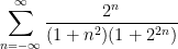
For instance, suppose one wanted to show that the sum

$\displaystyle \sum_{n=-\infty}^\infty \frac{2^n}{(1+n^2) (1+2^{2n})}$

was convergent. Lower bounding the denominator term ${1+2^{2n}}$ by ${1}$ or by ${2^{2n}}$ , one obtains the bounds

$\displaystyle \frac{2^n}{(1+n^2) (1+2^{2n})} \ll \frac{2^n}{1+n^2} \ \ \ \ \ (4)$

and also

$\displaystyle \frac{2^n}{(1+n^2) (1+2^{2n})} \ll \frac{2^n}{(1+n^2) 2^{2n}} = \frac{2^{-n}}{1+n^2} \ \ \ \ \ (5)$

so by applying (2) we obtain the unified bound

$\displaystyle \frac{2^n}{(1+n^2) (1+2^{2n})} \ll \frac{2^n}{(1+n^2) 2^{2n}} = \frac{\max(2^n,2^{-n})}{1+n^2}.$

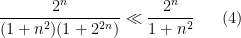
To deal with this bound, we can split into the two contributions ${n \geq 0}$ , where ${2^{-n}}$ dominates, and ${n < 0}$ , where ${2^n}$ dominates. In the former case we see (from the ratio test, for instance) that the sum

$\displaystyle \sum_{n=0}^\infty \frac{2^{-n}}{1+n^2}$

is absolutely convergent, and in the latter case we see that the sum

$\displaystyle \sum_{n=-\infty}^{-1} \frac{2^{n}}{1+n^2}$

is also absolutely convergent, so the entire sum is absolutely convergent. But once one has this argument, one can try to streamline it, for instance by taking the geometric mean of (4), (5) rather than the minimum to obtain the weaker bound

$\displaystyle \frac{2^n}{(1+n^2) (1+2^{2n})} \ll \frac{1}{1+n^2} \ \ \ \ \ (6)$

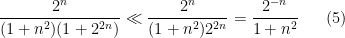
and now one can conclude without decomposition just by observing the absolute convergence of the doubly infinite sum ${\sum_{n=-\infty}^\infty \frac{1}{1+n^2}}$ . This is a less “efficient” estimate, because one has conceded a lot of the decay in the summand by using (6) (the summand used to be exponentially decaying in ${n}$ , but is now only polynomially decaying), but it is still sufficient for the purpose of establishing absolute convergence.

One of the key advantages of dealing with order of magnitude estimates, as opposed to sharp inequalities, is that the arithmetic becomes tropical. More explicitly, we have the important rule

$\displaystyle X + Y \asymp \max(X,Y)$

whenver ${X,Y}$ are non-negative, since we clearly have

$\displaystyle \max(X,Y) \leq X+Y \leq 2 \max(X,Y).$

In praticular, if ${Y \leq X}$ , then ${O(X) + O(Y) = O(X)}$ . That is to say, given two orders of magnitudes, any term ${O(Y)}$ of equal or lower order to a “main term” ${O(X)}$ can be discarded. This is a very useful rule to keep in mind when trying to estimate sums or integrals, as it allows one to discard many terms that are not contributing to the final answer. It also sets up the fundamental divide and conquer strategy for estimation: if one wants to prove a bound such as ${A \ll X}$ , it will suffice to obtain a decomposition

$\displaystyle A = A_1 + \dots + A_k$

or at least an upper bound

$\displaystyle A \ll A_1 + \dots + A_k$

of ${A}$ by some bounded number of components ${A_1,\dots,A_k}$ , and establish the bounds ${A_1 \ll X, \dots, A_k \ll X}$ separately. Typically the ${A_1,\dots,A_k}$ will be (morally at least) smaller than the original quantity ${A}$ – for instance, if ${A}$ is a sum of non-negative quantities, each of the ${A_i}$ might be a subsum of those same quantities – which means that such a decomposition is a “free move”, in the sense that it does not risk making the problem harder. (This is because, if the original bound ${A \ll X}$ is to be true, each of the new objectives ${A_1 \ll X, \dots, A_k \ll X}$ must also be true, and so the decomposition can only make the problem logically easier, not harder.) The only costs to such decomposition are that your proofs might be ${k}$ times longer, as you may be repeating the same arguments ${k}$ times, and that the implied constants in the ${A_1 \ll X, \dots, A_k \ll X}$ bounds may be worse than the implied constant in the original ${A \ll X}$ bound. However, in many cases these costs are well worth the benefits of being able to simplify the problem into smaller pieces. As mentioned above, once one successfully executes a divide and conquer strategy, one can go back and try to reduce the number of decompositions, for instance by unifying components that are treated by similar methods, or by replacing strong but unwieldy estimates with weaker, but more convenient estimates.

The above divide and conquer strategy does not directly apply when one is decomposing into an unbounded number of pieces ${A_j}$ , ${j=1,2,\dots}$ . In such cases, one needs an additional gain in the index ${j}$ that is summable in ${j}$ in order to conclude. For instance, if one wants to establish a bound of the form ${A \ll X}$ , and one has located a decomposition or upper bound

$\displaystyle A \ll \sum_{j=1}^\infty A_j$

that looks promising for the problem, then it would suffice to obtain exponentially decaying bounds such as

$\displaystyle A_j \ll 2^{-cj} X$

for all ${j \geq 1}$ and some constant ${c>0}$ , since this would imply

$\displaystyle A \ll \sum_{j=1}^\infty 2^{-cj} X \ll X \ \ \ \ \ (7)$

thanks to the geometric series formula. (Here it is important that the implied constants in the asymptotic notation are uniform on ${j}$ ; a ${j}$ -dependent bound such as ${A_j \ll_j 2^{-cj} X}$ would be useless for this application, as then the growth of the implied constant in ${j}$ could overwhelm the exponential decay in the ${2^{-cj}}$ factor). Exponential decay is in fact overkill; polynomial decay such as

$\displaystyle A_j \ll \frac{X}{j^{1+c}}$

would already be sufficient, although harmonic decay such

$\displaystyle A_j \ll \frac{X}{j} \ \ \ \ \ (8)$

is not quite enough (the sum ${\sum_{j=1}^\infty \frac{1}{j}}$ diverges logarithmically), although in many such situations one could try to still salvage the bound by working a lot harder to squeeze some additional logarithmic factors out of one’s estimates. For instance, if one can improve \eqre{ajx} to

$\displaystyle A_j \ll \frac{X}{j \log^{1+c} j}$

for all ${j \geq 2}$ and some constant ${c>0}$ , since (by the integral test) the sum ${\sum_{j=2}^\infty \frac{1}{j\log^{1+c} j}}$ converges (and one can treat the ${j=1}$ term separately if one already has (8)).

Sometimes, when trying to prove an estimate such as ${A \ll X}$ , one has identified a promising decomposition with an unbounded number of terms

$\displaystyle A \ll \sum_{j=1}^J A_j$

(where ${J}$ is finite but unbounded) but is unsure of how to proceed next. Often the next thing to do is to study the extreme terms ${A_1}$ and ${A_J}$ of this decomposition, and first try to establish (the presumably simpler) tasks of showing that ${A_1 \ll X}$ and ${A_J \ll X}$ . Often once one does so, it becomes clear how to combine the treatments of the two extreme cases to also treat the intermediate cases, obtaining a bound ${A_j \ll X}$ for each individual term, leading to the inferior bound ${A \ll JX}$ ; this can then be used as a starting point to hunt for additional gains, such as the exponential or polynomial gains mentioned previously, that could be used to remove this loss of ${J}$ . (There are more advanced techniques, such as those based on controlling moments such as the square function ${()\sum_{j=1}^J |A_j|^2)^{1/2}}$ , or trying to understand the precise circumstances in which a “large values” scenario ${|A_j| \gg X}$ occurs, and how these scenarios interact with each other for different ${j}$ , but these are beyond the scope of this post, as they are rarely needed when dealing with sums or integrals of elementary functions.)

— 1.1. Psychological distinctions between exact and asymptotic arithmetic —

The adoption of the “divide and conquer” strategy requires a certain mental shift from the “simplify, simplify” strategy that one is taught in high school algebra. In the latter strategy, one tries to collect terms in an expression make them as short as possible, for instance by working with a common denominator, with the idea that unified and elegant-looking expressions are “simpler” than sprawling expressions with many terms. In contrast, the divide and conquer strategy is intentionally extremely willing to greatly increase the total length of the expressions to be estimated, so long as each individual component of the expressions appears easier to estimate than the original one. Both strategies are still trying to reduce the original problem to a simpler problem (or collection of simpler sub-problems), but the metric by which one judges whether the problem has become simpler is rather different.

A related mental shift that one needs to adopt in analysis is to move away from the exact identities that are so prized in algebra (and in undergraduate calculus), as the precision they offer is often unnecessary and distracting for the task at hand, and often fail to generalize to more complicated contexts in which exact identities are no longer available. As a simple example, consider the task of estimating the expression

$\displaystyle \int_0^a \frac{dx}{1+x^2}$

where ${a > 0}$ is a parameter. With a trigonometric substitution, one can evaluate this expression exactly as ${\mathrm{arctan}(a)}$ , however the presence of the arctangent can be inconvenient if one has to do further estimation tasks (for instance, if ${a}$ depends in a complicated fashion on other parameters, which one then also wants to sum or integrate over). Instead, by observing the trivial bounds

$\displaystyle \int_0^a \frac{dx}{1+x^2} \leq \int_0^a\ dx = a$

and

$\displaystyle \int_0^a \frac{dx}{1+x^2} \leq \int_0^\infty\ \frac{dx}{1+x^2} = \frac{\pi}{2}$

one can combine them using (2) to obtain the upper bound

$\displaystyle \int_0^a \frac{dx}{1+x^2} \leq \min( a, \frac{\pi}{2} ) \asymp \min(a,1)$

and similar arguments also give the matching lower bound, thus

$\displaystyle \int_0^a \frac{dx}{1+x^2} \asymp \min(a,1). \ \ \ \ \ (9)$

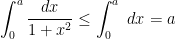
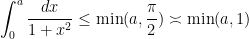
This bound, while cruder than the exact answer of ${\mathrm{arctan}(a)}$ , is often good enough for many applications (par ticularly in situations where one is willing to concede constants in the bounds), and can be more tractible to work with than the exact answer. Furthermore, these arguments can be adapted without difficulty to treat similar expressions such as

$\displaystyle \int_0^a \frac{dx}{(1+x^2)^\alpha}$

for any fixed exponent ${\alpha>0}$ , which need not have closed form exact expressions in terms of elementary functions such as the arctangent when ${\alpha}$ is non-integer.

As a general rule, instead of relying exclusively on exact formulae, one should seek approximations that are valid up to the degree of precision that one seeks in the final estimate. For instance, suppose one one wishes to establish the bound

$\displaystyle \sec(x) - \cos(x) = x^2 + O(x^3)$

for all sufficiently small ${x}$ . If one was clinging to the exact identity mindset, one could try to look for some trigonometric identity to simplify the left-hand side exactly, but the quicker (and more robust) way to proceed is just to use Taylor expansion up to the specified accuracy ${O(x^3)}$ to obtain

$\displaystyle \cos(x) = 1 - \frac{x^2}{2} + O(x^3)$

which one can invert using the geometric series formula ${(1-y)^{-1} = 1 + y + y^2 + \dots}$ to obtain

$\displaystyle \sec(x) = 1 + \frac{x^2}{2} + O(x^3)$

from which the claim follows. (One could also have computed the Taylor expansion of ${\sec(x)}$ directly, but as this is a series that is usually not memorized, this can take a little bit more time than just computing it directly to the required accuracy.) Note that the notion of “specified accuracy” may have to be interpreted in a relative sense if one is planning to multiply or divide several estimates together. For instance, if one wishes to establsh the bound

$\displaystyle \sin(x) \cos(x) = x + O(x^3)$

for small ${x}$ , one needs an approximation

$\displaystyle \sin(x) = x + O(x^3)$

to the sine function that is accurate to order ${O(x^3)}$ , but one only needs an approximation

$\displaystyle \cos(x) = 1 + O(x^2)$

to the cosine function that is accurate to order ${O(x^2)}$ , because the cosine is to be multiplied by ${\sin(x)= O(x)}$ . Here the key is to obtain estimates that have a relative error of ${O(x^2)}$ , compared to the main term (which is ${1}$ for cosine, and ${x}$ for sine).

The following table lists some common approximations that can be used to simplify expressions when one is only interested in order of magnitude bounds (with ${c>0}$ an arbitrary small constant):

The quantity… is comparable to … provided that… ${X+Y}$ ${X}$ ${0 \leq Y \ll X}$ or ${|Y| \leq X/2}$ ${\sin z}$ , ${\tan z}$ , ${e^{iz}-1}$ ${|z|}$ ${|z| \leq \frac{\pi}{2} - c}$ ${\cos z}$ ${1}$ ${|z| \leq \pi/2 - c}$ ${\sin x}$ ${\mathrm{dist}(x, \pi {\bf Z})}$ ${x}$ real ${e^{ix}-1}$ ${\mathrm{dist}(x, 2\pi {\bf Z})}$ ${x}$ real ${\mathrm{arcsin} x}$ ${|x|}$ ${|x| \leq 1-c}$ ${\log(1+x)}$ ${|x|}$ ${|x| \leq 1-c}$ ${e^z-1}$ , ${\sinh z}$ , ${\tanh z}$ ${|z|}$ ${|z| \leq \frac{\pi}{2}-c}$ ${\cosh z}$ ${1}$ ${|z| \leq \frac{\pi}{2}-c}$ ${\sinh x}$ , ${\cosh x}$ ${e^x}$ ${|x| \gg 1}$ ${\tanh x}$ ${\min(|x|, 1)}$ ${x}$ real ${(1+x)^a-1}$ ${a|x|}$ ${a \gg 1}$ , ${a |x| \ll 1}$ ${n!}$ ${n^n e^{-n} \sqrt{n}}$ ${n \geq 1}$ ${\Gamma(s)}$ ${|s^s e^{-s}| / |s|^{1/2}}$ ${|z| \gg 1}$ , ${|\mathrm{arg} z| \leq \frac{\pi}{2} - c}$ ${\Gamma(\sigma+it)}$ ${|t|^{\sigma-1/2} e^{-\pi |t|/2}}$ ${\sigma = O(1)}$ , ${|t| \gg 1}$

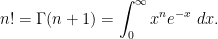
On the other hand, some exact formulae are still very useful, particularly if the end result of that formula is clean and tractable to work with (as opposed to involving somewhat exotic functions such as the arctangent). The geometric series formula, for instance, is an extremely handy exact formula, so much so that it is often desirable to control summands by a geometric series purely to use this formula (we already saw an example of this in (7)). Exact integral identities, such as

$\displaystyle \frac{1}{a} = \int_0^\infty e^{-at}\ dt$

or more generally

$\displaystyle \frac{\Gamma(s)}{a^s} = \int_0^\infty e^{-at} t^{s-1}\ dt$

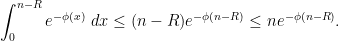
for ${a,s>0}$ (where ${\Gamma}$ is the Gamma function) are also quite commonly used, and fundamental exact integration rules such as the change of variables formula, the Fubini-Tonelli theorem or integration by parts are all esssential tools for an analyst trying to prove estimates. Because of this, it is often desirable to estimate a sum by an integral. The integral test is a classic example of this principle in action: a more quantitative versions of this test is the bound

$\displaystyle \int_{a}^{b+1} f(t)\ dt \leq \sum_{n=a}^b f(n) \leq \int_{a-1}^b f(t)\ dt \ \ \ \ \ (10)$

whenever ${a \leq b}$ are integers and ${f: [a-1,b+1] \rightarrow {\bf R}}$ is monotone decreasing, or the closely related bound

$\displaystyle \sum_{a \leq n \leq b} f(n) = \int_a^b f(t)\ dt + O( |f(a)| + |f(b)| ) \ \ \ \ \ (11)$

whenever ${a \geq b}$ are reals and ${f: [a,b] \rightarrow {\bf R}}$ is monotone (either increasing or decreasing); see Lemma 2 of this previous post. Such bounds allow one to switch back and forth quite easily between sums and integrals as long as the summand or integrand behaves in a mostly monotone fashion (for instance, if it is monotone increasing on one portion of the domain and monotone decreasing on the other). For more precision, one could turn to more advanced relationships between sums and integrals, such as the Euler-Maclaurin formula or the Poisson summation formula, but these are beyond the scope of this post.

Exercise 1 Suppose ${f: {\bf R} \rightarrow {\bf R}^+}$ obeys the quasi-monotonicity property ${f(x) \ll f(y)}$ whenever ${y-1 \leq x \leq y}$ . Show that ${\int_a^{b-1} f(t)\ dt \ll \sum_{n=a}^b f(n) \ll \int_a^{b+1} f(t)\ dt}$ for any integers ${a < b}$ .

Exercise 2 Use (11) to obtain the “cheap Stirling approximation”
$\displaystyle n! = \exp( n \log n - n + O(\log n) )$
for any natural number ${n \geq 2}$ . (Hint: take logarithms to convert the product ${n! = 1 \times 2 \times \dots \times n}$ into a sum.)

With practice, you will be able to identify any term in a computation which is already “negligible” or “acceptable” in the sense that its contribution is always going to lead to an error that is smaller than the desired accuracy of the final estimate. One can then work “modulo” these negligible terms and discard them as soon as they appear. This can help remove a lot of clutter in one’s arguments. For instance, if one wishes to establish an asymptotic of the form

$\displaystyle A = X + O(Y)$

for some main term ${X}$ and lower order error ${O(Y)}$ , any component of ${A}$ that one can already identify to be of size ${O(Y)}$ is negligible and can be removed from ${A}$ “for free”. Conversely, it can be useful to add negligible terms to an expression, if it makes the expression easier to work with. For instance, suppose one wants to estimate the expression

$\displaystyle \sum_{n=1}^N \frac{1}{n^2}. \ \ \ \ \ (12)$

This is a partial sum for the zeta function

$\displaystyle \sum_{n=1}^\infty \frac{1}{n^2} = \zeta(2) = \frac{\pi^2}{6}$

so it can make sense to add and subtract the tail ${\sum_{n=N+1}^\infty \frac{1}{n^2}}$ to the expression (12) to rewrite it as

$\displaystyle \frac{\pi^2}{6} - \sum_{n=N+1}^\infty \frac{1}{n^2}.$

To deal with the tail, we switch from a sum to the integral using (10) to bound

$\displaystyle \sum_{n=N+1}^\infty \frac{1}{n^2} \ll \int_N^\infty \frac{1}{t^2}\ dt = \frac{1}{N}$

giving us the reasonably accurate bound

$\displaystyle \sum_{n=1}^N \frac{1}{n^2} = \frac{\pi^2}{6} - O(\frac{1}{N}).$

One can sharpen this approximation somewhat using (11) or the Euler–Maclaurin formula; we leave this to the interested reader.

Another psychological shift when switching from algebraic simplification problems to estimation problems is that one has to be prepared to let go of constraints in an expression that complicate the analysis. Suppose for instance we now wish to estimate the variant

$\displaystyle \sum_{1 \leq n \leq N, \hbox{ square-free}} \frac{1}{n^2}$

of (12), where we are now restricting ${n}$ to be square-free. An identity from analytic number theory (the Euler product identity) lets us calculate the exact sum

$\displaystyle \sum_{n \geq 1, \hbox{ square-free}} \frac{1}{n^2} = \frac{\zeta(2)}{\zeta(4)} = \frac{15}{\pi^2}$

so as before we can write the desired expression as

$\displaystyle \frac{15}{\pi^2} - \sum_{n > N, \hbox{ square-free}} \frac{1}{n^2}.$

Previously, we applied the integral test (10), but this time we cannot do so, because the restriction to square-free integers destroys the monotonicity. But we can simply remove this restriction:

$\displaystyle \sum_{n > N, \hbox{ square-free}} \frac{1}{n^2} \leq \sum_{n > N} \frac{1}{n^2}.$

Heuristically at least, this move only “costs us a constant”, since a positive fraction ( ${1/\zeta(2)= 6/\pi^2}$ , in fact) of all integers are square-free. Now that this constraint has been removed, we can use the integral test as before and obtain the reasonably accurate asymptotic

$\displaystyle \sum_{1 \leq n \leq N, \hbox{ square-free}} \frac{1}{n^2} = \frac{15}{\pi^2} + O(\frac{1}{N}).$

— 2. More on decomposition —

The way in which one decomposes a sum or integral such as ${\sum_{n \in A} f(n)}$ or ${\int_A f(x)\ dx}$ is often guided by the “geometry” of ${f}$ , and in particular where ${f}$ is large or small (or whether various component terms in ${f}$ are large or small relative to each other). For instance, if ${f(x)}$ comes close to a maximum at some point ${x=x_0}$ , then it may make sense to decompose based on the distance ${|x-x_0|}$ to ${x_0}$ , or perhaps to treat the cases ${x \leq x_0}$ and ${x>x_0}$ separately. (Note that ${x_0}$ does not literally have to be the maximum in order for this to be a reasonable decomposition; if it is in “within reasonable distance” of the maximum, this could still be a good move. As such, it is often not worthwhile to try to compute the maximum of ${f}$ exactly, especially if this exact formula ends up being too complicated to be useful.)

If an expression involves a distance ${|X-Y|}$ between two quantities ${X,Y}$ , it is sometimes useful to split into the case ${|X| \leq |Y|/2}$ where ${X}$ is much smaller than ${Y}$ (so that ${|X-Y| \asymp |Y|}$ ), the case ${|Y| \leq |X|/2}$ where ${Y}$ is much smaller than ${X}$ (so that ${|X-Y| \asymp |X|}$ ), or the case when neither of the two previous cases apply (so that ${|X| \asymp |Y|}$ ). The factors of ${2}$ here are not of critical importance; the point is that in each of these three cases, one has some hope of simplifying the expression into something more tractable. For instance, suppose one wants to estimate the expression

$\displaystyle \int_{-\infty}^\infty \frac{dx}{(1+(x-a)^2) (1+(x-b)^2)} \ \ \ \ \ (13)$

in terms of the two real parameters ${a, b}$ , which we will take to be distinct for sake of this discussion. This particular integral is simple enough that it can be evaluated exactly (for instance using contour integration techniques), but in the spirit of Principle 1, let us avoid doing so and instead try to decompose this expression into simpler pieces. A graph of the integrand reveals that it peaks when ${x}$ is near ${a}$ or near ${b}$ . Inspired by this, one can decompose the region of integration into three pieces:

(i) The region where ${|x-a| \leq \frac{|a-b|}{2}}$ .
(ii) The region where ${|x-b| \leq \frac{|a-b|}{2}}$ .
(iii) The region where ${|x-a|, |x-b| > \frac{|a-b|}{2}}$ .

(This is not the only way to cut up the integral, but it will suffice. Often there is no “canonical” or “elegant” way to perform the decomposition; one should just try to find a decomposition that is convenient for the problem at hand.)

The reason why we want to perform such a decomposition is that in each of the three cases, one can simplify how the integrand depends on ${x}$ . For instance, in region (i), we see from the triangle inequality that ${|x-b|}$ is now comparable to ${|a-b|}$ , so that this contribution to (13) is comparable to

$\displaystyle \asymp \int_{|x-a| \leq |a-b|/2} \frac{dx}{(1+(x-a)^2) (1+(a-b)^2)}.$

Using a variant of (9), this expression is comparable to

$\displaystyle \asymp \min( 1, |a-b|/2) \frac{1}{1+(a-b)^2} \asymp \frac{\min(1, |a-b|)}{1+(a-b)^2}. \ \ \ \ \ (14)$

The contribution of region (ii) can be handled similarly, and is also comparable to (14). Finally, in region (iii), we see from the triangle inequality that ${|x-a|, |x-b|}$ are now comparable to each other, and so the contribution of this region is comparable to

$\displaystyle \asymp \int_{|x-a|, |x-b| > |a-b|/2} \frac{dx}{(1+(x-a)^2)^2}.$

Now that we have centered the integral around ${x=a}$ , we will discard the ${|x-b| > |a-b|/2}$ constraint, upper bounding this integral by

$\displaystyle \asymp \int_{|x-a| > |a-b|/2} \frac{dx}{(1+(x-a)^2)^2}.$

On the one hand this integral is bounded by

$\displaystyle \int_{-\infty}^\infty \frac{dx}{(1+(x-a)^2)^2} = \int_{-\infty}^\infty \frac{dx}{(1+x^2)^2} \asymp 1$

and on the other hand we can bound

$\displaystyle \int_{|x-a| > |a-b|/2} \frac{dx}{(1+(x-a)^2)^2} \leq \int_{|x-a| > |a-b|/2} \frac{dx}{(x-a)^4} \asymp |a-b|^{-3}$

and so we can bound the contribution of (iii) by ${O( \min( 1, |a-b|^{-3} ))}$ . Putting all this together, and dividing into the cases ${|a-b| \leq 1}$ and ${|a-b| > 1}$ , one can soon obtain a total bound of ${O(\min( 1, |a-b|^{-3}))}$ for the entire integral. One can also adapt this argument to show that this bound is sharp up to constants, thus

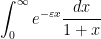
$\displaystyle \int_{-\infty}^\infty \frac{dx}{(1+(x-a)^2) (1+(x-b)^2)} \asymp \min( 1, |a-b|^{-3}) \asymp \frac{1}{1+|a-b|^3}.$

A powerful and common type of decomposition is dyadic decomposition. If the summand or integrand involves some quantity ${Q}$ in a key way, it is often useful to break up into dyadic regions such as ${2^{j-1} \leq Q < 2^{j}}$ , so that ${Q \sim 2^j}$ , and then sum over ${j}$ . (One can tweak the dyadic range ${2^{j-1} \leq Q < 2^{j}}$ here with minor variants such as ${2^{j} < Q \leq 2^{j+1}}$ , or replace the base ${2}$ by some other base, but these modifications mostly have a minor aesthetic impact on the arguments at best.) For instance, one could break up a sum

$\displaystyle \sum_{n=1}^{\infty} f(n) \ \ \ \ \ (15)$

into dyadic pieces

$\displaystyle \sum_{j=1}^\infty \sum_{2^{j-1} \leq n < 2^{j}} f(n)$

and then seek to estimate each dyadic block ${\sum_{2^{j-1} \leq n < 2^{j}} f(n)}$ separately (hoping to get some exponential or polynomial decay in ${j}$ ). The classical technique of Cauchy condensation is a basic example of this strategy. But one can also dyadically decompose other quantities than ${n}$ . For instance one can perform a “vertical” dyadic decomposition (in contrast to the “horizontal” one just performed) by rewriting (15) as

$\displaystyle \sum_{k \in {\bf Z}} \sum_{n \geq 1: 2^{k-1} \leq f(n) < 2^k} f(n);$

since the summand ${f(n)}$ is ${\asymp 2^k}$ , we may simplify this to

$\displaystyle \asymp \sum_{k \in {\bf Z}} 2^k \# \{ n \geq 1: 2^{k-1} \leq f(n) < 2^k\}.$

This now converts the problem of estimating the sum (15) to the more combinatorial problem of estimating the size of the dyadic level sets ${\{ n \geq 1: 2^{k-1} \leq f(n) < 2^k\}}$ for various ${k}$ . In a similar spirit, we have

$\displaystyle \int_A f(x)\ dx \asymp \sum_{k \in {\bf Z}} 2^k | \{ x \in A: 2^{k-1} \leq f(x) < 2^k \}|$

where ${|E|}$ denotes the Lebesgue measure of a set ${E}$ , and now we are faced with a geometric problem of estimating the measure of some explicit set. This allows one to use geometric intuition to solve the problem, instead of multivariable calculus:

Exercise 3 Let ${S}$ be a smooth compact submanifold of ${{\bf R}^d}$ . Establish the bound
$\displaystyle \int_{B(0,C)} \frac{dx}{\varepsilon^2 + \mathrm{dist}(x,S)^2} \ll \varepsilon$
for all ${0 < \varepsilon < C}$ , where the implied constants are allowed to depend on ${C, d, S}$ . (This can be accomplished either by a vertical dyadic decomposition, or a dyadic decomposition of the quantity ${\mathrm{dist}(x,S)}$ .)

Exercise 4 Solve problem (ii) from the introduction to this post by dyadically decomposing in the ${d}$ variable.

Remark 5 By such tools as (10), (11), or Exercise 1, one could convert the dyadic sums one obtains from dyadic decomposition into integral variants. However, if one wished, one could “cut out the middle-man” and work with continuous dyadic decompositions rather than discrete ones. Indeed, from the integral identity
$\displaystyle \int_0^\infty 1_{\lambda < Q \leq 2\lambda} \frac{d\lambda}{\lambda} = \log 2$
for any ${Q>0}$ , together with the Fubini–Tonelli theorem, we obtain the continuous dyadic decomposition
$\displaystyle \sum_{n \in A} f(n) = \int_0^\infty \sum_{n \in A: \lambda \leq Q(n) < 2\lambda} f(n)\ \frac{d\lambda}{\lambda}$
for any quantity ${Q(n)}$ that is positive whenever ${f(n)}$ is positive. Similarly if we work with integrals ${\int_A f(x)\ dx}$ rather than sums. This version of dyadic decomposition is occasionally a little more convenient to work with, particularly if one then wants to perform various changes of variables in the ${\lambda}$ parameter which would be tricky to execute if this were a discrete variable.

— 3. Exponential weights —

Many sums involve expressions that are “exponentially large” or “exponentially small” in some parameter. A basic rule of thumb is that any quantity that is “exponentially small” will likely give a negligible contribution when compared against quantities that are not exponentially small. For instance, if an expression involves a term of the form ${e^{-Q}}$ for some non-negative quantity ${Q}$ , which can be bounded on at least one portion of the domain of summation or integration, then one expects the region where ${Q}$ is bounded to provide the dominant contribution. For instance, if one wishes to estimate the integral

$\displaystyle \int_0^\infty e^{-\varepsilon x} \frac{dx}{1+x}$

for some ${0 < \varepsilon < 1/2}$ , this heuristic suggests that the dominant contribution should come from the region ${x = O(1/\varepsilon)}$ , in which one can bound ${e^{-\varepsilon x}}$ simply by ${1}$ and obtain an upper bound of

$\displaystyle \ll \int_{x = O(1/\varepsilon)} \frac{dx}{1+x} \ll \log \frac{1}{\varepsilon}.$

To make such a heuristic precise, one can perform a dyadic decomposition in the exponential weight ${e^{-\varepsilon x}}$ , or equivalently perform an additive decomposition in the exponent ${\varepsilon x}$ , for instance writing

$\displaystyle \int_0^\infty e^{-\varepsilon x} \frac{dx}{1+x} = \sum_{j=1}^\infty \int_{j-1 \leq \varepsilon x < j} e^{-\varepsilon x} \frac{dx}{1+x}.$

Exercise 6 Use this decomposition to rigorously establish the bound
$\displaystyle \int_0^\infty e^{-\varepsilon x} \frac{dx}{1+x} \ll \log \frac{1}{\varepsilon}$
for any ${0 < \varepsilon < 1/2}$ .

Exercise 7 Solve problem (i) from the introduction to this post.

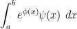
More generally, if one is working with a sum or integral such as

$\displaystyle \sum_{n \in A} e^{\phi(n)} \psi(n)$

$\displaystyle \int_A e^{\phi(x)} \psi(x)\ dx$

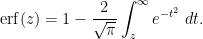
with some exponential weight ${e^\phi}$ and a lower order amplitude ${\psi}$ , then one typically expects the dominant contribution to come from the region where ${\phi}$ comes close to attaining its maximal value. If this maximum is attained on the boundary, then one typically has geometric series behavior away from the boundary, and one can often get a good estimate by obtaining geometric series type behavior. For instance, suppose one wants to estimate the error function

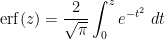
$\displaystyle \mathrm{erf}(z) = \frac{2}{\sqrt{\pi}} \int_0^z e^{-t^2}\ dt$

for ${z \geq 1}$ . In view of the complete integral

$\displaystyle \int_0^\infty e^{-t^2}\ dt = \frac{\sqrt{\pi}}{2}$

we can rewrite this as

$\displaystyle \mathrm{erf}(z) = 1 - \frac{2}{\sqrt{\pi}} \int_z^\infty e^{-t^2}\ dt.$

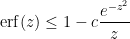
The exponential weight ${e^{-t^2}}$ attains its maximum at the left endpoint ${t=z}$ and decays quickly away from that endpoint. One could estimate this by dyadic decomposition of ${e^{-t^2}}$ as discussed previously, but a slicker way to proceed here is to use the convexity of ${t^2}$ to obtain a geometric series upper bound

$\displaystyle e^{-t^2} \leq e^{-z^2 - 2 z (t-z)}$

for ${t \geq z}$ , which on integration gives

$\displaystyle \int_z^\infty e^{-t^2}\ dt \leq \int_z^\infty e^{-z^2 - 2 z (t-z)}\ dt = \frac{e^{-z^2}}{2z}$

giving the asymptotic

$\displaystyle \mathrm{erf}(z) = 1 - O( \frac{e^{-z^2}}{z})$

for ${z \geq 1}$ .

Exercise 8 In the converse direction, establish the upper bound
$\displaystyle \mathrm{erf}(z) \leq 1 - c \frac{e^{-z^2}}{z}$
for some absolute constant ${c>0}$ and all ${z \geq 1}$ .

Exercise 9 If ${\theta n \leq m \leq n}$ for some ${1/2 < \theta < 1}$ , show that
$\displaystyle \sum_{k=m}^n \binom{n}{k} \ll \frac{1}{2\theta-1} \binom{n}{m}.$
(Hint: estimate the ratio between consecutive binomial coefficients ${\binom{n}{k}}$ and then control the sum by a geometric series).

When the maximum of the exponent ${\phi}$ occurs in the interior of the region of summation or integration, then one can get good results by some version of <a href="https://en.wikipedia.org/wiki/Laplace

$\displaystyle \int_a^b e^{\phi(x)} \psi(x)\ dx$

where ${\phi}$ attains a non-degenerate global maximum at some interior point ${x = x_0}$ . The rule of thumb here is that

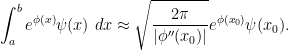$\displaystyle \int_a^b e^{\phi(x)} \psi(x)\ dx \approx \sqrt{\frac{2\pi}{|\phi''(x_0)|}} e^{\phi(x_0)} \psi(x_0).$

The heuristic justification is as follows. The main contribution should be when ${x}$ is close to ${x_0}$ . Here we can perform a Taylor expansion

$\displaystyle \phi(x) \approx \phi(x_0) - \frac{1}{2} |\phi''(x_0)| (x-x_0)^2$

since at a non-degenerate maximum we have ${\phi'(x_)=0}$ and ${\phi''(x_0) > 0}$ . Also, if ${\psi}$ is continuous, then ${\psi(x) \approx \psi(x_0)}$ when ${x}$ is close to ${x_0}$ . Thus we should be able to estimate the above integral by the gaussian integral

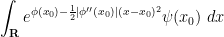
$\displaystyle \int_{\bf R} e^{\phi(x_0) - \frac{1}{2} |\phi''(x_0)| (x-x_0)^2} \psi(x_0)\ dx$

which can be computed to equal ${\sqrt{\frac{2\pi}{|\phi''(x_0)|}} e^{\phi(x_0)} \psi(x_0)}$ as desired.

Let us illustrate how this argument can be made rigorous by considering the task of estimating the factorial ${n!}$ of a large number. In contrast to what we did in Exercise \ref”>, we will proceed using a version of Laplace’s method, relying on the integral representation

$\displaystyle n! = \Gamma(n+1) = \int_0^\infty x^n e^{-x}\ dx.$

As ${n}$ is large, we will consider ${x^n}$ to be part of the exponential weight rather than the amplitude, writing this expression as

$\displaystyle \int_0^\infty e^{-\phi(x)}\ dx$

where

$\displaystyle \phi(x) = x - n \log x.$

The function ${\phi}$ attains a global maximum at ${x_0 = n}$ , with ${\phi(n) = 0}$ and ${\phi''(n) = 1/n}$ . We will therefore decompose this integral into three pieces

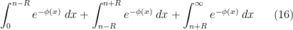
$\displaystyle \int_0^{n-R} e^{-\phi(x)}\ dx + \int_{n-R}^{n+R} e^{-\phi(x)}\ dx + \int_{n+R}^\infty e^{-\phi(x)}\ dx \ \ \ \ \ (16)$

where ${0 < R < n}$ is a radius parameter which we will choose later, as it is not immediately obvious for now how to select it.

The main term is expected to be the middle term, so we shall use crude methods to bound the other two terms. For the first part where ${0 < x \leq n-R}$ , ${\phi}$ is increasing so we can crudely bound ${e^{-\phi(x)} \leq e^{-\phi(n-R)}}$ and thus

$\displaystyle \int_0^{n-R} e^{-\phi(x)}\ dx \leq (n-R) e^{-\phi(n-R)} \leq n e^{-\phi(n-R)}.$

(We expect ${R}$ to be much smaller than ${n}$ , so there is not much point to saving the tiny ${-R}$ term in the ${n-R}$ factor.) For the third part where ${x \geq n+R}$ , ${\phi}$ is decreasing, but bounding ${e^{-\phi(x)}}$ by ${e^{-\phi(n+R)}}$ would not work because of the unbounded nature of ${x}$ ; some additional decay is needed. Fortunately, we have a strict increase

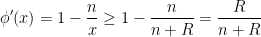$\displaystyle \phi'(x) = 1 - \frac{n}{x} \geq 1 - \frac{n}{n+R} = \frac{R}{n+R}$

for ${x \geq n+R}$ , so by the intermediate value theorem we have

$\displaystyle \phi(x) \geq \phi(n+R) + \frac{R}{n+R} (x-n-R)$

and after a short calculation this gives

$\displaystyle \int_{n+R}^\infty e^{-\phi(x)}\ dx \leq \frac{n+R}{R} e^{-\phi(n+R)} \ll \frac{n}{R} e^{-\phi(n+R)}.$

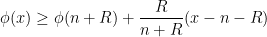
Now we turn to the important middle term. If we assume ${R \leq n/2}$ , then we will have ${\phi'''(x) = O( 1/n^2 )}$ in the region 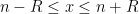${n-R \leq x \leq n+R}$ , so by Taylor’s theorem with remainder

$\displaystyle \phi(x) = \phi(n) + \phi'(n) (x-n) + \frac{1}{2} \phi''(n) (x-n)^2 + O( \frac{|x-n|^3}{n^2} )$

$\displaystyle = \phi(n) + \frac{(x-n)^2}{2n} + O( \frac{R^3}{n^2} ).$

If we assume that ${R = O(n^{2/3})}$ , then the error term is bounded and we can exponentiate to obtain

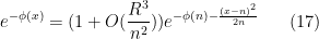$\displaystyle e^{-\phi(x)} = (1 + O(\frac{R^3}{n^2})) e^{-\phi(n) - \frac{(x-n)^2}{2n}} \ \ \ \ \ (17)$

for ${n-R \leq x \leq n+R}$ and hence

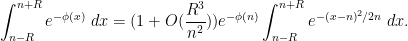
$\displaystyle \int_{n-R}^{n+R} e^{-\phi(x)}\ dx = (1 + O(\frac{R^3}{n^2})) e^{-\phi(n)} \int_{n-R}^{n+R} e^{-(x-n)^2/2n}\ dx.$

If we also assume that ${R \gg \sqrt{n}}$ , we can use the error function type estimates from before to estimate

$\displaystyle \int_{n-R}^{n+R} e^{-(x-n)^2/2n}\ dx = \sqrt{2\pi n} + O( \frac{n}{R} e^{-R^2/2n} ).$

Putting all this together, and using \eqref for details.

Exercise 10 Solve problem (iii) from the introduction. (Hint: extract out the term ${\frac{k^{2n-4k}}{(n-k)^{2n-4k}}}$ to write as the exponential factor ${e^{\phi(k)}}$ , placing all the other terms (which are of polynomial size) in the amplitude function ${\psi(k)}$ . The function ${\phi}$ will then attain a maximum at ${k=n/2}$ ; perform a Taylor expansion and mimic the arguments above.)