The Kepler Problem (Part 2)
Azimuth 2025-07-14
I’ve been working on a math project involving the periodic table of elements and the Kepler problem—that is, the problem of a particle moving in an inverse square force law. I started it in 2021, but I just finished. I want to explain it. But I need some things to be fresh in your mind, so I’m going to republish some old blog articles, starting with this one. (For Part 1 go here, but you won’t need that for what’s to come.)
Let’s start with the ‘eccentricity vector’. This is a conserved quantity for the Kepler problem. It was named the ‘Runge–Lenz vector’ after Lenz used it in 1924 to study the hydrogen atom in the framework of the ‘old quantum mechanics’ of Bohr and Sommerfeld: Lenz cite Runge’s popular German textbook on vector analysis from 1919, which explains this vector. But Runge never claimed any originality: he attributed this vector to Gibbs, who wrote about it in his book on vector analysis in 1901!
Nowadays many people call it the ‘Laplace–Runge–Lenz vector’, honoring Laplace’s discussion of it in his famous treatise on celestial mechaics in 1799. But in fact this vector goes back at least to Jakob Hermann, who wrote about it in 1710, triggering further work on this topic by Johann Bernoulli in the same year.
Nobody has seen signs of this vector in work before Hermann. So, we might call it the Hermann–Bernoulli–Laplace–Gibbs–Runge–Lenz vector, or just the Hermann vector. But I prefer to call it the eccentricity vector, because for a particle in an inverse square law its magnitude is the eccentricity of that orbit!
Let’s suppose we have a particle whose position 

where I remove the arrow from a vector when I want to talk about its magnitude. So, I’m setting the mass of this particle equal to 1, along with the constant saying the strength of the force. That’s because I want to keep the formulas clean! With these conventions, the momentum of the particle is

For this system it’s well-known that the following energy is conserved:

as well as the angular momentum vector:

But the interesting thing for me today is the eccentricity vector:

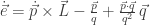
Let’s check that it’s conserved! Taking its time derivative,

But angular momentum is conserved so the second term vanishes, and

so we get
But the inverse square force law says

so

How can we see that this vanishes? Mind you, there are various geometrical ways to think about this, but today I’m in the mood for checking that my skills in vector algebra are sufficient for a brute-force proof—and I want to record this proof so I can see it later!
To get anywhere we need to deal with the cross product in the above formula:
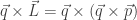
There’s a nice identity for the vector triple product:

I could have fun talking about why this is true, but I won’t now! I’ll just use it:

and plug this into our formula
getting
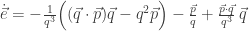
But look—everything cancels! So

and the eccentricity vector is conserved!
So, it seems that the inverse square force law has 7 conserved quantities: the energy 


The first of these relations is pretty obvious: 

But wait, why are they at right angles? Because
The first term is orthogonal to 


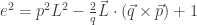
The second relation is a lot less obvious, but also more interesting. Let’s take the dot product of

or in other words,

But remember this nice cross product identity:

Since 

so

Then we can use the cyclic identity for the scalar triple product:

to rewrite this as
or simply

or even better,

But this means that

which is our second relation between conserved quantities for the Kepler problem!
This relation makes a lot of sense if you know that 
• if 

• if 

• if 

But why is


Using the cyclic property of the scalar triple product we can rewrite this as

Now, we know that 


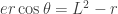
or

This is well-known, at least among students of physics who have solved the Kepler problem, to be the equation of a conic of eccentricity
Another thing that’s good to do is define a rescaled eccentricity vector. In the case of elliptical orbits, where 

Then we can take our relation
and rewrite it as
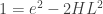
and then divide by 

or
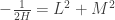
This suggests an interesting similarity between 

For now, you might try this:
• Wikipedia, Laplace–Runge–Lenz vector.
and of course this: