The Kepler Problem (Part 3)

Azimuth 2025-07-16

The Kepler problem studies a particle moving in an inverse square force, like a planet orbiting the Sun. Last time I talked about an extra conserved quantity associated to this problem, which keeps elliptical orbits from precessing or changing shape. This extra conserved quantity is sometimes called the Laplace–Runge–Lenz vector, but since it was first discovered by none of these people, I prefer to call it the ‘eccentricity vector’

In 1847, Hamilton noticed a fascinating consequence of this extra conservation law. For a particle moving in an inverse square force, its momentum moves along a circle!

Greg Egan has given a beautiful geometrical argument for this fact:

• Greg Egan, The ellipse and the atom.

I will not try to outdo him; instead I’ll follow a more dry, calculational approach. One reason is that I’m trying to amass a little arsenal of formulas connected to the Kepler problem.

Let’s dive in. Remember from last time: we’re studying a particle whose position $\vec q$ obeys

$\ddot{\vec q} = - \frac{\vec q}{q^3}$

Its momentum is

$\vec p = m \dot{\vec q}$

Its momentum is not conserved. Its conserved quantities are energy:

$E = \frac{1}{2} p^2 - \frac{1}{q}$

the angular momentum vector:

$\vec L = \vec q \times \vec p$

and the eccentricity vector:

$\vec e = \vec p \times \vec L - \frac{\vec q}{q}$

Now for the cool part: we can show that

$\displaystyle{ \left( \vec p - \frac{\vec L \times \vec e}{L^2} \right)^2 = \frac{1}{L^2} }$

Thus, the momentum $\vec p$ stays on a circle of radius $1/L$ centered at the point $(\vec L \times \vec e)/L^2.$ And since $\vec L$ and $\vec e$ are conserved, this circle doesn’t change! Let’s call it Hamilton’s circle.

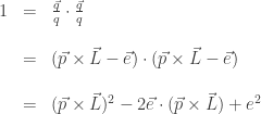
Now let’s actually do the calculations needed to show that the momentum stays on Hamilton’s circle. Since

$\vec e = \vec p \times \vec L - \frac{\vec q}{q}$

we have

$\frac{\vec q}{q} = \vec p \times \vec L - \vec e$

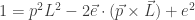
Taking the dot product of this vector with itself, which is 1, we get

$\begin{array}{ccl} 1 &=& \frac{\vec q}{q} \cdot \frac{\vec q}{q} \\ \\ &=& (\vec p \times \vec L - \vec e) \cdot (\vec p \times \vec L - \vec e) \\ \\ &=& (\vec p \times \vec L)^2 - 2 \vec e \cdot (\vec p \times \vec L) + e^2 \end{array}$

Now, notice that $\vec p$ and $\vec L$ are orthogonal since $\vec L = \vec q \times \vec p.$ Thus

$(\vec p \times \vec L)^2 = p^2 L^2$

I actually used this fact and explained it in more detail last time. Substituting this in, we get

$1 = p^2 L^2 - 2 \vec e \cdot (\vec p \times \vec L) + e^2$

Similarly, $\vec e$ and $\vec L$ are orthogonal! After all,

$\vec e = \vec p \times \vec L - \frac{\vec q}{q}$

The first term is orthogonal to $\vec L$ since it’s the cross product of $\vec L$ and some other vector. And the second term is orthogonal to $\vec L$ since $\vec L$ is the cross product of $\vec q$ and some other vector! So, we have

$(\vec L \times \vec e)^2 = L^2 e^2$

and thus

$\displaystyle { e^2 = \frac{(\vec L \times \vec e)^2}{L^2} }$

Substituting this in, we get

$\displaystyle { 1 = p^2 L^2 - 2 \vec e \cdot (\vec p \times \vec L) + \frac{(\vec L \times \vec e)^2}{L^2} }$

Using the cyclic property of the scalar triple product, we can rewrite this as

$\displaystyle { 1 = p^2 L^2 - 2 \vec p \cdot (\vec L \times \vec e) + \frac{(\vec L \times \vec e)^2}{L^2} }$

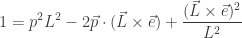
This is nicer because it involves $\vec L \times \vec e$ in two places. If we divide both sides by $L^2$ we get

$\displaystyle { \frac{1}{L^2} = p^2 - \frac{2}{L^2} \; \vec p \cdot (\vec L \times \vec e) + \frac{(\vec L \times \vec e)^2}{L^4} }$

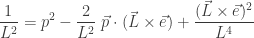
And now for the final flourish! The right hand is the dot product of a vector with itself:

$\displaystyle { \frac{1}{L^2} = \left(\vec p - \frac{\vec L \times \vec e}{L^2}\right)^2 }$

This is the equation for Hamilton’s circle!

Now, beware: the momentum $\vec p$ doesn’t usually move at a constant rate along Hamilton’s circle, since that would force the particle’s orbit to itself be circular.

But on the bright side, the momentum moves along Hamilton’s circle regardless of whether the particle’s orbit is elliptical, parabolic or hyperbolic. And we can easily distinguish the three cases using Hamilton’s circle!

After all, the center of Hamilton’s circle is the point $(\vec L \times \vec e)/L^2,$ and

$(\vec L \times \vec e)^2 = L^2 e^2$

so the distance of this center from the origin is

$\displaystyle{ \sqrt{\frac{(\vec L \times \vec e)^2}{L^4}} = \sqrt{\frac{L^2 e^2}{L^4}} = \frac{e}{L} }$

On the other hand, the radius of Hamilton’s circle is $1/L.$ So his circle encloses the origin, goes through the origin or does not enclose the origin depending on whether $e < 1, e = 1$ or $e > 1.$ But we saw last time that these three cases correspond to elliptical, parabolic and hyperbolic orbits!

Summarizing:

• If $e < 1$ the particle’s orbit is an ellipse and the origin lies inside Hamilton’s circle. The momentum goes round and round Hamilton’s circle as time passes.

• If $e = 1$ the particle’s orbit is a parabola and the origin lies exactly on Hamilton’s circle. The particle’s momentum approaches zero as time approaches $\pm \infty,$ so its momentum goes around Hamilton’s circle exactly once as time passes.

• If $e > 1$ the particle’s orbit is a hyperbola and the origin lies outside Hamilton’s circle. The particle’s momentum approaches distinct nonzero values as time approaches $\pm \infty,$ so its momentum goes around just a portion of Hamilton’s circle.

By the way, in general the curve traced out by the momentum vector of a particle is called a hodograph. So you can learn more about Hamilton’s circle with the help of that buzzword.