The Kepler Problem (Part 12)

Azimuth 2025-10-15

It’s been a while. Let me finally wrap up this this series. I’ll show you how we can the periodic table of elements from a quantum field theory of massless spin-1/2 particles.

We’ve been studying the hydrogen atom using Schrödinger’s equation, but still taking the electron’s spin into account. This is more realistic than the basic Schrödinger equation that ignores spin, but less realistic than a full-fledged relativistic treatment using the Dirac equation. It’s a pretty good approximation. We saw that bound states of this hydrogen atom can be reinterpreted as states of a massless left-handed spin-1/2 particle in the Einstein universe—a universe where space is the 3-sphere $S^3.$

Then I ‘second quantized’ both theories. If we do this to the massless spin-1/2 particle, we get a free quantum field theory on the Einstein universe! This describes arbitrary collections of noninteracting massless spin-1/2 particles. If we second quantize the hydrogen atom, we get a theory of multi-electron atoms—but a naive theory where the electrons don’t interact. In this naive theory we don’t get the periodic table of elements. But today I want to tweak the Hamiltonian so we do get the observed periodic table, at least roughly.

Let’s do it!

In Part 7 we saw how the Hilbert space of bound states of the hydrogen atom, taking the electron’s spin into account, is

$\mathcal{H} = L^2(S^3) \otimes \mathbb{C}^2$

In atomic physics, the eigenspaces of the Hamiltonian $H$ on $\mathcal{H}$ are called shells, while the joint eigenspaces of the operators $H$ and the angular momentum squared, $L^2,$ are called subshells. We denote the shells as

$\displaystyle{ \mathcal{H}_n = \{ \psi \in \mathcal{H} \; H\psi = -\frac{1}{2n^2} \psi \} }$

and the subshells as

$\mathcal{H}_{n,\ell} = \{ \psi \in \mathcal{H}_n : \; L^2 \psi = \ell(\ell + 1) \psi \}$

The shells are direct sums of subshells as follows:

$\mathcal{H}_n = \bigoplus_{\ell = 0}^{n-1} \mathcal{H}_{n,\ell}$

and the direct sum of all the shells is the whole Hilbert space of bound states of the hydrogen atom:

$\mathcal{H} = \bigoplus_{n = 1}^\infty \mathcal{H}_n$

The dimension of the subshell $\mathcal{H}_{n,\ell}$ is $2(2\ell + 1),$ so the dimension of the shell $\mathcal{H}_n$ is

$2(1 + 3 + 5 + \cdots + (2n - 1)) = 2n^2$

In Part 11 we second quantized the hydrogen atom and got the fermionic Fock space $\mathbf{\Lambda} \mathcal{H}$ which describes collections of electrons bound to the nucleus. This suggests that we could understand the periodic table this way!

The Aufbau principle is a famous approximate way to describe the ground state of an $N$ -electron atom as a state $\phi$ in the $N$ -particle subspace of the Fock space $\mathbf{\Lambda} \mathcal{H}.$ To do this, we choose a Hamiltonian $H_{\text{Fock}}$ on $\mathbf{\Lambda} \mathcal{H}$ and decree that $\phi$ must minimize the expected energy $\langle \phi , H_{\text{Fock}}\, \phi \rangle$ among all unit vectors in the $N$ -particle subspace. However, we choose the Hamiltonian $H_{\text{Fock}}$ in a very simplistic way. We ignore the details of electron-electron interactions! Instead, we simply assign an energy $E_{n,\ell}$ to each subshell, let $H_{\text{single}}$ be the unique Hamiltonian on $\mathcal{H}$ such that

$\psi \in \mathcal{H}_{n,\ell} \implies H_{\text{single}} \psi = E_{n,\ell} \,\psi$

and then we let

$H_{\text{Fock}} = d\mathbf{\Lambda}(H_{\text{single}})$

Thus, $H_{\text{Fock}}$ has a basis of eigenvectors that are wedge products of single-particle states lying in various subshells. Explicitly, if

$\phi = \psi_1 \wedge \cdots \wedge \psi_N$ where $\psi_i \in \mathcal{H}_{n_i, \ell_i}$

then we have

$H_{\text{Fock}} \, \phi = (E_{n_1,\ell_1} + \cdots + E_{n_N, \ell_N}) \phi$

Thus, we can minimize $\langle \phi , H_{\text{Fock}}\, \phi \rangle$ among unit vectors in the $N$ -particle subspace by choosing $N$ distinct basis vectors

$\psi_i = |n_i, \ell_i, m_i, s_i \rangle$

in a way that minimizes the total energy $E_{n_1,\ell_1} + \cdots + E_{n_N, \ell_N}.$

If we follow this recipe taking $H_{\text{single}}$ to be the hydrogen atom Hamiltonian $H,$ we get results that do not closely match the observed periodic table of elements. With this choice we get energies

$\displaystyle{ E_{n,\ell} = -\frac{1}{2n^2} }$

that depend only on the shell, not the subshell. Thus, this choice makes no prediction about the order in which subshells are filled! That’s no good.

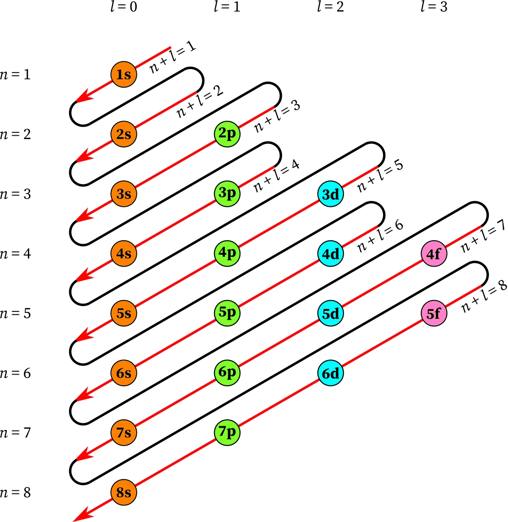
For the recipe to give results that more closely match the periodic table, we need to choose the energies $E_{n,\ell}$ in a more clever way. In 1936, Madelung argued for these rules:

• subshells are filled in order of increasing value of $n + \ell$ ;

• for subshells with the same value of $n + \ell,$ subshells are filled in order of decreasing $\ell$ (or equivalently, increasing $n$ ).

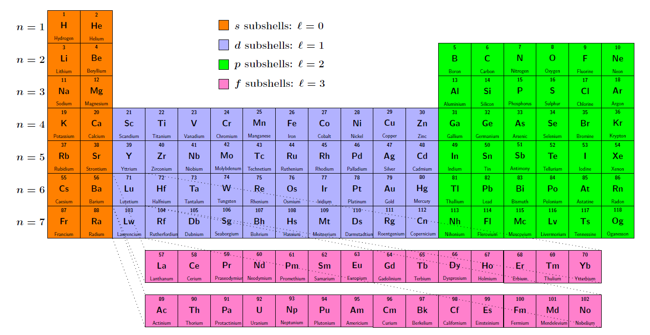
In reality this nice pattern is broken by quite a few elements, but here we only consider a simple model in which the Madelung rules hold. The pattern of subshell filling then looks like this:

The above chart uses some old but still popular notation from spectroscopy:

• $\ell = 0$ : $s$ • $\ell = 1$ : $p$ • $\ell = 2$ : $d$ • $\ell = 3$ : $f$

For example, the subshell $\mathcal{H}_{3,2}$ is denoted $3d$ while $\mathcal{H}_{5,3}$ is denoted $5f.$

In 1945, a chemist named Wiswesser noted that the Madelung rules follow from the recipe we outlined if we choose

$E_{n,\ell} = n + \ell - \frac{\ell}{\ell + 1}$

There are many other functions of $n$ and $\ell$ that achieve the same effect. For example, we can also obtain the Madelung rules if we take

$E_{n,\ell} = 2n + (2\ell + 1) + (2\ell + 1)^{-1}$

and this formula is more convenient for us.

The Madelung rules do not always hold! The first exception is element 24, chromium. The Madelung rules predict that chromium has 2 electrons in the $4s$ subshell and 4 electrons in the $3d$ subshell, while in fact it has 1 in the $4s$ and 5 in the $3d.$ There are other exceptions. Nonetheless the general structure of the periodic table seems to be in reasonably good accord with the Madelung rules for all the elements studied chemically so far, though relativistic effects may end this for very heavy elements.

Thus it is of some interest, if only as a curiosity, to define a Hamiltonian on the Hilbert space $\mathcal{H}$ that takes the eigenvalue $E_{n,\ell}$ in the subshell $\mathcal{H}_{n,\ell}.$ These energies are not at all close to the actual energies of the various multi-electron atoms, and any monotone function of $E_{n,\ell}$ would also give the Madelung rules—but this particular Hamiltonian is fairly simple.

Recall from Part 7:

$\begin{array}{cclll} A^2 |n , \ell, m \rangle &=& \frac{1}{4}(n^2 - 1) |n , \ell, m, s \rangle \\ [3pt] L^2 |n , \ell, m \rangle &=& \ell(\ell + 1) |n , \ell, m, s \rangle \end{array}$

The Duflo isomorphism, as discussed in Part 6, makes it natural to define operators

$\tilde{A}^2 = A^2 + \frac{1}{4}, \qquad \tilde{L}^2 = L^2 + \frac{1}{4}$

If we then define $\tilde{A}$ and $\tilde{L}$ to be the square roots of these operators, we have

$\begin{array}{cclcl} \tilde{A} |n , \ell, m \rangle &=& \frac{1}{2} n |n , \ell, m \rangle \\ [3pt] \tilde{L} |n , \ell, m \rangle &=& (\ell + \frac{1}{2}) |n , \ell, m \rangle \end{array}$

and thus

$(2\tilde{A} + 2\tilde{L} + (2\tilde{L})^{-1})|n , \ell, m, s \rangle = E_{n,\ell} |n , \ell, m, s\rangle$

This suggests taking our single-particle Hamiltonian to be

$H_{\text{single}} = 2\tilde{A} + 2\tilde{L} + (2\tilde{L})^{-1}$

If we then define a Hamiltonian on the Fock space $\mathbf{\Lambda} \mathcal{H}$ by

$H_{\text{Fock}} = d\mathbf{\Lambda}(H_{\text{single}})$

and create an orthonormal basis $\psi_i$ of eigenvectors of $H_{\text{Fock}},$ listed in order of increasing eigenvalue, these eigenvectors correspond to the elements with subshells filled as predicted by the Madelung rules. The one exception is the state $\psi_0$ with no electrons, sometimes called ‘element zero’ and identified with the neutron. For example:

$\begin{array}{ccll} \psi_1 &=& |1,0,0,\frac{1}{2} \rangle & \text{hydrogen} \\ \\ \psi_2 &=& |1,0,0,\frac{1}{2} \rangle \wedge |1,0,0,-\frac{1}{2}\rangle & \text{helium} \\ \\ \psi_3 &=& |1,0,0,\frac{1}{2} \rangle \wedge |1,0,0,-\frac{1}{2}\rangle \wedge |2,0,0,\frac{1}{2}\rangle & \text{lithium} \end{array}$

and so on.

Here the assignments of magnetic quantum numbers $m$ and spins $s$ are not determined by the rules we have laid out. These are governed, at least approximately, by Hund’s rules:

• every $m$ state in a subshell is singly occupied before any is doubly occupied;

• all of the electrons in singly occupied orbitals have the same spin.

We could go further and attempt to choose a simple Hamiltonian for which the principle of energy mimization also gives Hund’s rules. However, we prefer to stop here, leaving you with the challenge of finding a better-behaved quantum field theory on the Einstein universe whose Hamiltonian gives the Madelung rules, or perhaps better understanding the Hamiltonian we have given here.

Here is the periodic table we get from our approach:

and here are the energies for subshells

$E_{n,\ell} = 2n + (2\ell + 1) + (2\ell + 1)^{-1}$

that we’re using in our approach:

For more, read my paper:

• Second quantization for the Kepler problem.

or these blog articles, which are more expository and fun:

• Part 1: a quick overview of Kepler’s work on atoms and the solar system, and more modern developments.

• Part 2: why the eccentricity vector is conserved for a particle in an inverse square force, and what it means.

• Part 3: why the momentum of a particle in an inverse square force moves around in a circle.

• Part 4: why the 4d rotation group $\text{SO}(4)$ acts on bound states of a particle in an attractive inverse square force.

• Part 5: quantizing the bound states of a particle in an attractive inverse square force, and getting the Hilbert space $L^2(S^3)$ for bound states of a hydrogen atom, neglecting the electron’s spin.

• Part 6: how the Duflo isomorphism explains quantum corrections to the hydrogen atom Hamiltonian.

• Part 7: why the Hilbert space of bound states for a hydrogen atom including the electron’s spin is $L^2(S^3) \otimes \mathbb{C}^2.$

• Part 8: why $L^2(S^3) \otimes \mathbb{C}^2$ is also the Hilbert space for a massless spin-1/2 particle in the Einstein universe.

• Part 9: a quaternionic description of the hydrogen atom’s bound states (a digression not needed for later parts).

• Part 10: changing the complex structure on $L^2(S^3) \otimes \mathbb{C}^2$ to eliminate negative-energy states of the massless spin-1/2 particle, as often done.

• Part 11: second quantizing the massless spin-1/2 particle and getting a quantum field theory on the Einstein universe, or alternatively a theory of collections of electrons orbiting a nucleus.

• Part 12: obtaining the periodic table of elements from a quantum field theory on the Einstein universe.