Agent-Based Models (Part 7)

Azimuth 2024-02-29

Last time I presented a simple, limited class of agent-based models where each agent independently hops around a graph. I wrote:

Today the probability for an agent to hop from one vertex of the graph to another by going along some edge will be determined the moment the agent arrives at that vertex. It will depend only on the agent and the various edges leaving that vertex. Later I’ll want this probability to depend on other things too—like whether other agents are at some vertex or other. When we do that, we’ll need to keep updating this probability as the other agents move around.

Let me try to figure out that generalization now.

Last time I discovered something surprising to me. To describe it, let’s bring in some jargon. The conditional probability per time of an agent making a transition from its current state to a chosen other state (given that it doesn’t make some other transition) is called the hazard function of that transition. In a Markov process, the hazard function is actually a constant, independent of how long the agent has been in its current state. In a semi-Markov process, the hazard function is a function only of how long the agent has been in its current state.

For example, people like to describe radioactive decay using a Markov process, since experimentally it doesn’t seem that ‘old’ radioactive atoms decay at a higher or lower rate than ‘young’ ones. (Quantum theory says this can’t be exactly true, but nobody has seen deviations yet.) On the other hand, the death rate of people is highly non-Markovian, but we might try to describe it using a semi-Markov process. Shortly after birth it’s high—that’s called ‘infant mortality’. Then it goes down, and then it gradually increases.

We definitely want to our agent-based processes to have the ability to describe semi-Markov processes. What surprised me last time is that I could do it without explicitly keeping track of how long the agent has been in its current state, or when it entered its current state!

The reason is that we can decide which state an agent will transition to next, and when, as soon as it enters its current state. This decision is random, of course. But using random number generators we can make this decision the moment the agent enters the given state—because there is nothing more to be learned by waiting! I described an algorithm for doing this.

I’m sure this is well-known, but I had fun rediscovering it.

But today I want to allow the hazard function for a given agent to make a given transition to depend on the states of other agents. In this case, if some other agent randomly changes state, we will need to recompute our agent’s hazard function. There is probably no computationally feasible way to avoid this, in general. In some analytically solvable models there might be—but we’re simulating systems precisely because we don’t know how to solve them analytically.

So now we’ll want to keep track of the residence time of each agent—that is, how long it’s been in its current state. But William Waites pointed out a clever way to do this: it’s cheaper to keep track of the agent’s arrival time, i.e. when it entered its current state. This way you don’t need to keep updating the residence time. Whenever you need to know the residence time, you can just subtract the arrival time from the current clock time.

Even more importantly, our model should now have ‘informational links’ from states to transitions. If we want the presence or absence of agents in some state to affect the hazard function of some transition, we should draw a ‘link’ from that state to that transition! Of course you could say that anything is allowed to affect anything else. But this would create an undisciplined mess where you can’t keep track of the chains of causation. So we want to see explicit ‘links’.

So, here’s my new modeling approach, which generalizes the one we saw last time. For starters, a model should have:

• a finite set $V$ of vertices or states,

• a finite set $E$ of edges or transitions,

• maps $u, d \colon E \to V$ mapping each edge to its source and target, also called its upstream and downstream,

• finite set $A$ of agents,

• a finite set $L$ of links,

• maps $s \colon L \to V$ and $t \colon L \to E$ mapping each edge to its source (a state) and its target (a transition).

All of this stuff, except for the set of agents, is exactly what we had in our earlier paper on stock-flow models, where we treated people en masse instead of as individual agents. You can see this in Section 2.1 here:

• John Baez, Xiaoyan Li, Sophie Libkind, Nathaniel D. Osgood, Evan Patterson, Compositional modeling with stock and flow models.

So, I’m trying to copy that paradigm, and eventually unify the two paradigms as much as possible.

But they’re different! In particular, our agent-based models will need a ‘jump function’. This says when each agent $a \in A$ will undergo a transition $e \in E$ if it arrives at the state upstream to that transition at a specific time $t \in \mathbb{R}.$ This jump function will not be deterministic: it will be a stochastic function, just as it was in yesterday’s formalism. But today it will depend on more things! Yesterday it depended only on $a, e$ and $t.$ But now the links will come into play.

For each transition $e \in E$ , there is set of links whose target is that transition, namely

$t^{-1}(e) = \{\ell \in L \; \vert \; t(\ell) = e \}$

Each link in $\ell \in t^{-1}(e)$ will have one state $v$ as its source. We say this state affects the transition $e$ via the link $\ell.$

We want the jump function for the transition $e$ to depend on the presence or absence of agents in each state that affects this transition.

Which agents are in a given state? Well, it depends! But those agents will always form some subset of $A,$ and thus an element of $2^A.$ So, we want the jump function for the transition $e$ to depend on an element of

$\prod_{\ell \in t^{-1}(e)} 2^A = 2^{A \times t^{-1}(e)}$

I’ll call this element $S_e.$ And as mentioned earlier, the jump function will also depend on a choice of agent $a \in A$ and on the arrival time of the agent $a.$

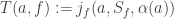
So, we’ll say there’s a jump function $j_e$ for each transition $e,$ which is a stochastic function

$j_e \colon A \times 2^{A \times t^{-1}(e)} \times \mathbb{R} \rightsquigarrow \mathbb{R}$

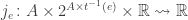
The idea, then, is that $j_e(a, S_e, t)$ is the answer to this question:

If at time $t$ agent $a$ arrived at the vertex $u(e),$ and the agents at states linked to the edge $e$ are described by the set $S_e,$ when will agent $a$ move along the edge $e$ to the vertex $d(e),$ given that it doesn’t do anything else first?

The answer to this question can keep changing as agents other than $a$ move around, since the set $S$ can keep changing. This is the big difference between today’s formalism and yesterday’s.

Here’s how we run our model. At every moment in time we keep track of some information about each agent $a \in A,$ namely:

• Which vertex is it at now? We call this vertex the agent’s state, $\sigma(a).$

• When did it arrive at this vertex? We call this time the agent’s arrival time, $\alpha(a).$

• For each edge $e$ whose upstream is $\sigma(a),$ when will agent $a$ move along this edge if it doesn’t do anything else first? Call this time $T(a,e).$

I need to explain how we keep updating these pieces of information (supposing we already have them). Let’s assume that at some moment in time $t_i$ an agent makes a transition. More specifically, suppose agent $\underline{a} \in A$ makes a transition $\underline{e}$ from the state

$\underline{v} = u(\underline{e}) \in V$

to the state

$\underline{v}' = d(\underline{e}) \in V.$

At this moment we update the following information:

1) We set

$\alpha(\underline{a}) = t_i$

(So, we update the arrival time of that agent.)

2) We set

$\sigma(\underline{a}) := \underline{v}'$

(So, we update the state of that agent.)

3) We recompute the subset of agents in the state $\underline{v}$ (by removing $\underline{a}$ from this subset) and in the state $\underline{v}'$ (by adding $\underline{a}$ to this subset).

4) For every transition $f$ that’s affected by the state $\underline{v}$ or the state $\underline{v}'$ , and for every agent $a$ in the upstream state of that transition, we set

$T(a,f) := j_f(a, S_f, \alpha(a))$

where $S_f$ is the element of $2^{A \times t^{-1}(f)}$ saying which subset of agents is in each state affecting the transition $f.$ (So, we update our table of times at which agent $a$ will make the transition $f,$ given that it doesn’t do anything else first.)

Now we need to compute the next time at which something happens, namely $t_{i+1}.$ And we need to compute what actually happens then!

To do this, we look through our table of times $T(a,e)$ for each agent $a$ and all transitions out of the state that agent is in. and see which time is smallest. If there’s a tie, break it. Then we reset $\underline{a}$ and $\underline{e}$ to be the agent-edge pair that minimizes $T(a,e).$

5) We set

$t_{i+1} := T(\underline{a},\underline{e})$

Then we loop back around to step 1), but with $i+1$ replacing $i.$

Whew! I hope you followed that. If not, please ask questions.